Stochastic Differential Equations (SDEs)

• Wikipedia: Stochastic Differential Equations

• SDE example

• RODE example

Stochastic Differential Equations (SDEs)

• Recommended SDE solvers: https://docs.sciml.ai/DiffEqDocs/stable/solvers/sde_solve/

Scalar SDEs with one state variable

Solving the equation: \(du=f(u,p,t)dt + g(u,p,t)dW\)

• \(f(u,p,t)\) is the ordinary differential equations (ODEs) part

• \(g(u,p,t)\) is the stochastic part, paired with a Brownian motion term \(dW\).

using StochasticDiffEq
using Plots

ODE function

f = (u, p, t) -> p.α * u

#1 (generic function with 1 method)

Noise term

g = (u, p, t) -> p.β * u

#3 (generic function with 1 method)

Setup the SDE problem

p = (α=1, β=1)
u0 = 1 / 2
dt = 1 // 2^(4)
tspan = (0.0, 1.0)
prob = SDEProblem(f, g, u0, (0.0, 1.0), p)

SDEProblem with uType Float64 and tType Float64. In-place: false
Non-trivial mass matrix: false
timespan: (0.0, 1.0)
u0: 0.5

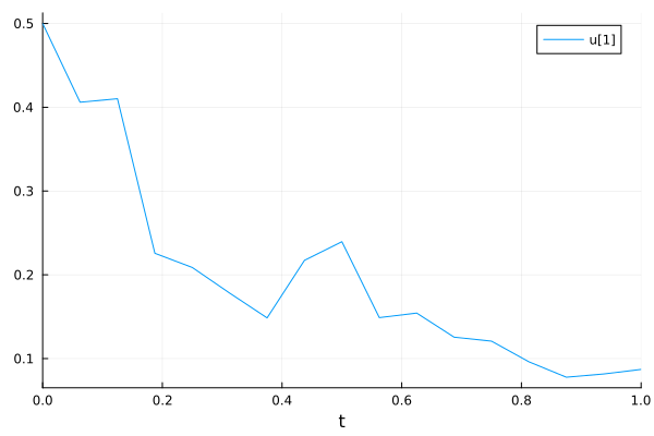
Use the classic Euler-Maruyama algorithm to solve the problem

sol = solve(prob, EM(), dt=dt)

retcode: Success
Interpolation: 1st order linear
t: 17-element Vector{Float64}:
 0.0
 0.0625
 0.125
 0.1875
 0.25
 0.3125
 0.375
 0.4375
 0.5
 0.5625
 0.625
 0.6875
 0.75
 0.8125
 0.875
 0.9375
 1.0
u: 17-element Vector{Float64}:
 0.5
 0.4060141951150904
 0.4101897966898335
 0.2256598988116713
 0.20874660426723934
 0.17813737710215408
 0.14856604429004105
 0.21730900729349048
 0.23952888756391175
 0.1489098725630178
 0.1543256690094215
 0.12554770558240397
 0.1208157193443121
 0.0961428560066162
 0.07777383657359958
 0.08163501836437098
 0.08709107299710533

Visualize

plot(sol)

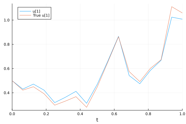
The analytical solution: If \(f(u,p,t) = \alpha u\) and \(g(u,p,t) = \beta u\), the analytical solution is \(u(t, W_t) = u_0 exp((\alpha - \frac{\beta^2}{2})t + \beta W_t)\)

f_analytic = (u0, p, t, W) -> u0 * exp((p.α - (p.β^2) / 2) * t + p.β * W)
ff = SDEFunction(f, g, analytic=f_analytic)
prob = SDEProblem(ff, g, u0, (0.0, 1.0), p)

SDEProblem with uType Float64 and tType Float64. In-place: false
Non-trivial mass matrix: false
timespan: (0.0, 1.0)
u0: 0.5

Visualize numerical and analytical solutions

sol = solve(prob, EM(), dt=dt)
plot(sol, plot_analytic=true)

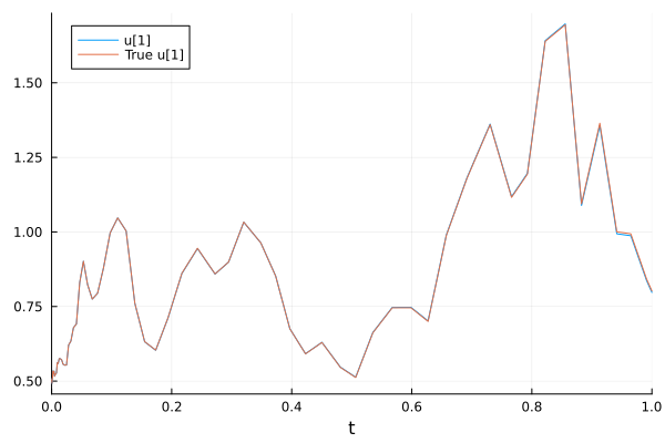
Use a higher-order adaptive solver SRIW1() for a more accurate result

sol = solve(prob, SRIW1())
plot(sol, plot_analytic=true)

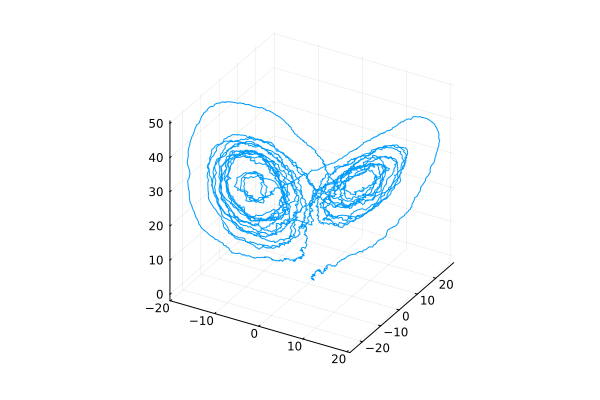
SDEs with diagonal Noise

Each state variable are influenced by its own noise. Here we use the Lorenz system with noise as an example.

using StochasticDiffEq
using Plots

function lorenz!(du, u, p, t)
    du[1] = 10.0(u[2] - u[1])
    du[2] = u[1] * (28.0 - u[3]) - u[2]
    du[3] = u[1] * u[2] - (8 / 3) * u[3]
end

function σ_lorenz!(du, u, p, t)
    du[1] = 3.0
    du[2] = 3.0
    du[3] = 3.0
end

prob_sde_lorenz = SDEProblem(lorenz!, σ_lorenz!, [1.0, 0.0, 0.0], (0.0, 20.0))
sol = solve(prob_sde_lorenz, SRIW1())
plot(sol, idxs=(1, 2, 3), label=false)

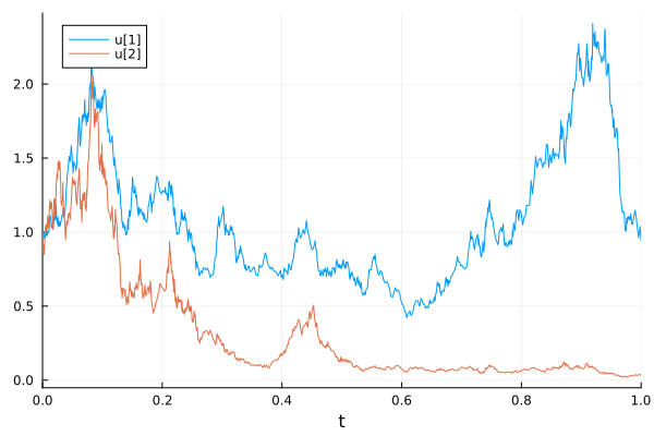
SDEs with scalar Noise

The same noise process (W) is applied to all state variables.

using StochasticDiffEq
using DiffEqNoiseProcess: WienerProcess
using Plots

Exponential growth with noise

f = (du, u, p, t) -> (du .= u)
g = (du, u, p, t) -> (du .= u)

#9 (generic function with 1 method)

Problem setup

u0 = rand(4, 2)
W = WienerProcess(0.0, 0.0, 0.0)
prob = SDEProblem(f, g, u0, (0.0, 1.0), noise=W)

SDEProblem with uType Matrix{Float64} and tType Float64. In-place: true
Non-trivial mass matrix: false
timespan: (0.0, 1.0)
u0: 4×2 Matrix{Float64}:
 0.0704615  0.656255
 0.740109   0.511136
 0.0120195  0.218462
 0.627732   0.291875

Solve and visualize

sol = solve(prob, SRIW1())
plot(sol)

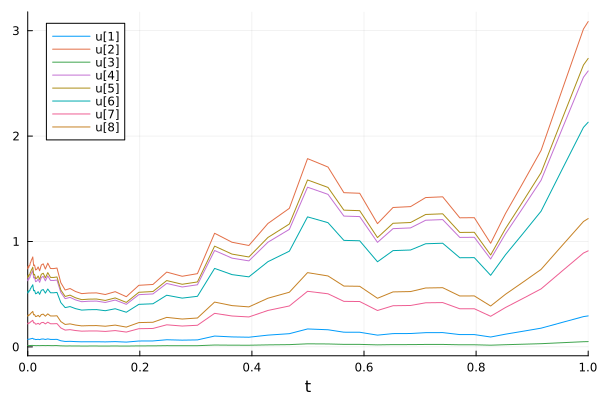
SDEs with Non-Diagonal (matrix) Noise

A more general type of noise allows for the terms to linearly mixed via noise function g being a matrix.

\[\begin{split} \begin{aligned} du_1 &= f_1(u,p,t)dt + g_{11}(u,p,t)dW_1 + g_{12}(u,p,t)dW_2 + g_{13}(u,p,t)dW_3 + g_{14}(u,p,t)dW_4 \\ du_2 &= f_2(u,p,t)dt + g_{21}(u,p,t)dW_1 + g_{22}(u,p,t)dW_2 + g_{23}(u,p,t)dW_3 + g_{24}(u,p,t)dW_4 \end{aligned} \end{split}\]

using StochasticDiffEq
using Plots

f = (du, u, p, t) -> du .= 1.01u

g = (du, u, p, t) -> begin
    du[1, 1] = 0.3u[1]
    du[1, 2] = 0.6u[1]
    du[1, 3] = 0.9u[1]
    du[1, 4] = 0.12u[1]
    du[2, 1] = 1.2u[2]
    du[2, 2] = 0.2u[2]
    du[2, 3] = 0.3u[2]
    du[2, 4] = 1.8u[2]
end

u0 = ones(2)
tspan = (0.0, 1.0)

(0.0, 1.0)

The noise matrix itself is determined by the keyword argument noise_rate_prototype

prob = SDEProblem(f, g, u0, tspan, noise_rate_prototype=zeros(2, 4))
sol = solve(prob, LambaEulerHeun())
plot(sol)

Random ODEs

https://docs.sciml.ai/DiffEqDocs/stable/tutorials/rode_example/

Random ODEs (RODEs) is a more general form that allows nonlinear mixings of randomness.

\(du = f(u, p, t, W) dt\) where \(W(t)\) is a Wiener process (Gaussian process).

RODEProblem(f, u0, tspan [, params]) constructs an RODE problem.

The model function signature is

• f(u, p, t, W) (out-of-place form).

• f(du, u, p, t, W) (in-place form).

using StochasticDiffEq
using Plots

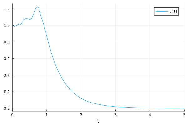
Scalar RODEs

u0 = 1.00
tspan = (0.0, 5.0)
prob = RODEProblem((u, p, t, W) -> 2u * sin(W), u0, tspan)
sol = solve(prob, RandomEM(), dt=1 / 100)
plot(sol)

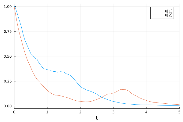
Systems of RODEs

function f4(du, u, p, t, W)
    du[1] = 2u[1] * sin(W[1] - W[2])
    du[2] = -2u[2] * cos(W[1] + W[2])
end

u0 = [1.00; 1.00]
tspan = (0.0, 5.0)

prob = RODEProblem(f4, u0, tspan)
sol = solve(prob, RandomEM(), dt=1 / 100)
plot(sol)

---

This notebook was generated using Literate.jl.