ModelingToolkit: define ODEs with symbolic expressions

ModelingToolkit: define ODEs with symbolic expressions#

You can also define ODE systems symbolically using ModelingToolkit.jl (MTK) and let MTK generate high-performance ODE functions.

transforming and simplifying expressions for performance
Jacobian and Hessian generation
accessing eliminated states (called observed variables)
building and connecting subsystems programmatically (component-based modeling)

Radioactive decay#

Here we use the same example of decaying radioactive elements

using ModelingToolkit
using OrdinaryDiffEq
using Plots

independent variable (time) and dependent variables

@independent_variables t
@variables c(t) RHS(t)

\[\begin{split} \begin{equation} \left[ \begin{array}{c} c\left( t \right) \\ \mathtt{RHS}\left( t \right) \\ \end{array} \right] \end{equation} \end{split}\]

parameters: decay rate

@parameters λ

\[\begin{split} \begin{equation} \left[ \begin{array}{c} \lambda \\ \end{array} \right] \end{equation} \end{split}\]

Differential operator w.r.t. time

D = Differential(t)

Differential(t)

Equations in MTK use the tilde character (~) for equality. Every MTK system requires a name. The @named macro simply ensures that the symbolic name matches the name in the REPL.

eqs = [
    RHS ~ -λ * c
    D(c) ~ RHS
]

\[\begin{split} \begin{align} \mathtt{RHS}\left( t \right) &= - c\left( t \right) \lambda \\ \frac{\mathrm{d} c\left( t \right)}{\mathrm{d}t} &= \mathtt{RHS}\left( t \right) \end{align} \end{split}\]

Build and ODE system from equations

@mtkbuild sys = ODESystem(eqs, t)

\[ \begin{align} \frac{\mathrm{d} c\left( t \right)}{\mathrm{d}t} &= \mathtt{RHS}\left( t \right) \end{align} \]

Setup initial conditions, time span, parameter values, the ODEProblem, and solve the problem.

p = [λ => 1.0]
u0 = [c => 1.0]
tspan = (0.0, 2.0)
prob = ODEProblem(sys, u0, tspan, p);
sol = solve(prob)

retcode: Success
Interpolation: 3rd order Hermite
t: 8-element Vector{Float64}:
 0.0
 0.10001999200479662
 0.34208427066999536
 0.6553980136343391
 1.0312652525315806
 1.4709405856363595
 1.9659576669700232
 2.0
u: 8-element Vector{Vector{Float64}}:
 [1.0]
 [0.9048193287657775]
 [0.7102883621328676]
 [0.5192354400036404]
 [0.35655576576996556]
 [0.2297097907863828]
 [0.14002247272452764]
 [0.1353360028400881]

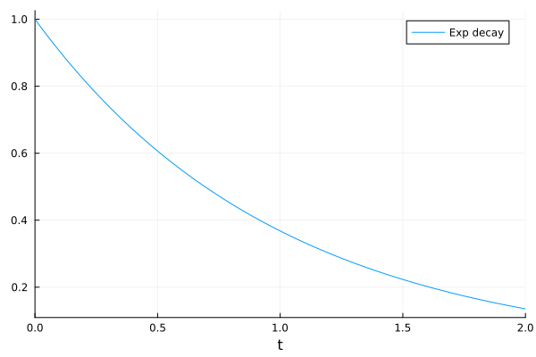
Visualize the solution

plot(sol, label="Exp decay")

../_images/ca7c012538e49660eb46d7971458b53e17561a928a4dd8cc9379f56b5e0ef578.png

The solution interface provides symbolic access. You can access the results of c directly.

sol[c]

8-element Vector{Float64}:
0
9048193287657775
7102883621328676
5192354400036404
35655576576996556
2297097907863828
14002247272452764
1353360028400881

With interpolations with specified time points

sol(0.0:0.1:2.0, idxs=c)

t: 0.0:0.1:2.0
u: 21-element Vector{Float64}:
0
9048374180989603
8187305973051514
7408182261974484
670319782243577
6065302341562359
5488116548085096
49658509875978446
4493280239179766
4065692349272286
 ⋮
30119273799114377
2725309051375336
24659717503493142
22313045099430742
20189530933816474
18268185222253558
16529821250790575
14956912660454402
13533600284008812

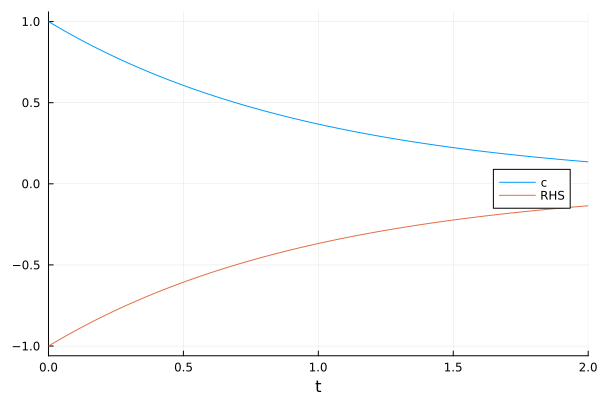
The eliminated term (RHS in this example) is still traceable.

plot(sol, idxs=[c, RHS], legend=:right)

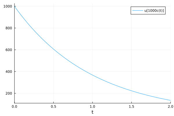
../_images/018d3d12fc2503c9110f6270410e0a22c616fac9e3a887d0deddbc3cea0278ff.png

The indexing interface allows symbolic calculations.

plot(sol, idxs=[c * 1000])

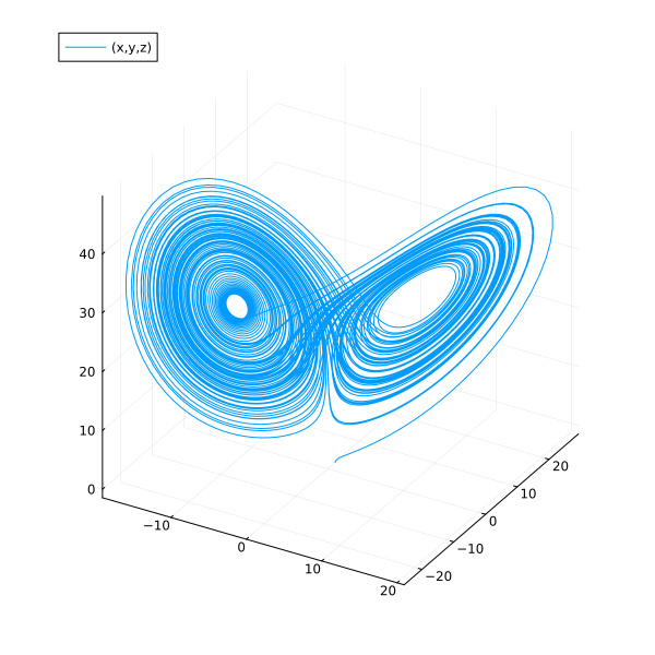
../_images/c5c85ca653ea17566dc1763a5eac504b7dad431157a7868d5e7d45fed6de9cb8.png

Lorenz system#

Here we setup the initial conditions and parameters with default values.

@independent_variables t
@variables x(t) = 1.0 y(t) = 0.0 z(t) = 0.0
@parameters (σ=10.0, ρ=28.0, β=8 / 3)

D = Differential(t)

eqs = [
    D(x) ~ σ * (y - x)
    D(y) ~ x * (ρ - z) - y
    D(z) ~ x * y - β * z
]

@mtkbuild sys = ODESystem(eqs, t)

\[\begin{split} \begin{align} \frac{\mathrm{d} x\left( t \right)}{\mathrm{d}t} &= \left( - x\left( t \right) + y\left( t \right) \right) \sigma \\ \frac{\mathrm{d} y\left( t \right)}{\mathrm{d}t} &= - y\left( t \right) + x\left( t \right) \left( - z\left( t \right) + \rho \right) \\ \frac{\mathrm{d} z\left( t \right)}{\mathrm{d}t} &= x\left( t \right) y\left( t \right) - z\left( t \right) \beta \end{align} \end{split}\]

Here we are using default values, so we pass empty arrays for initial conditions and parameter values.

tspan = (0.0, 100.0)
prob = ODEProblem(sys, [], tspan, []);
sol = solve(prob)

retcode: Success
Interpolation: 3rd order Hermite
t: 1292-element Vector{Float64}:
   0.0
   3.5678604836301404e-5
   0.0003924646531993154
   0.003262408731175873
   0.009058076622686189
   0.01695647090176743
   0.027689960116420883
   0.041856352219618344
   0.060240411865493296
   0.08368541210909924
   ⋮
  99.43545175575305
  99.50217600300971
  99.56297541572351
  99.62622492183432
  99.69561088424294
  99.77387244562912
  99.86354266863755
  99.93826978918452
 100.0
u: 1292-element Vector{Vector{Float64}}:
 [1.0, 0.0, 0.0]
 [0.9996434557625105, 0.0009988049817849058, 1.781434788799189e-8]
 [0.9961045497425811, 0.010965399721242457, 2.1469553658389193e-6]
 [0.9693591548287857, 0.0897706331002921, 0.00014380191884671585]
 [0.9242043547708632, 0.24228915014052968, 0.0010461625485930237]
 [0.8800455783133068, 0.43873649717821195, 0.003424260078582332]
 [0.8483309823046307, 0.6915629680633586, 0.008487625469885364]
 [0.8495036699348377, 1.0145426764822272, 0.01821209108471829]
 [0.9139069585506618, 1.442559985646147, 0.03669382222358562]
 [1.0888638225734468, 2.0523265829961646, 0.07402573595703686]
 ⋮
 [1.2013409155396158, -2.429012698730855, 25.83593282347909]
 [-0.4985909866565941, -2.2431908075030083, 21.591758421186338]
 [-1.3554328352527145, -2.5773570617802326, 18.48962628032902]
 [-2.1618698772305467, -3.5957801801676297, 15.934724265473792]
 [-3.433783468673715, -5.786446127166032, 14.065327938066913]
 [-5.971873646288483, -10.261846004477597, 14.060290896024572]
 [-10.941900618598972, -17.312154206417734, 20.65905960858999]
 [-14.71738043327772, -16.96871551014668, 33.06627229408802]
 [-13.714517151605754, -8.323306384833089, 38.798231477265624]

Phase plot w.r.t symbols.

plot(sol, idxs=(x, y, z), size=(600, 600))

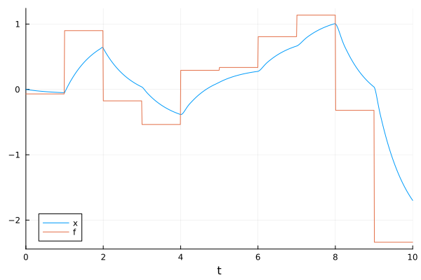
../_images/877d23eb27833008ff9a469f2137d536f544346145a3c443d5ba95aa1acbab61.png

Non-autonomous ODEs#

Sometimes a model might have a time-variant external force, which is too complex or impossible to express it symbolically. In such situation, one could apply @register_symbolic to it to exclude it from symbolic transformations and use it numerically.

@independent_variables t
@variables x(t) f(t)
@parameters τ
D = Differential(t)

Differential(t)

Define a time-dependent random external force

value_vector = randn(10)
f_fun(t) = t >= 10 ? value_vector[end] : value_vector[Int(floor(t))+1]

f_fun (generic function with 1 method)

“Register” arbitrary Julia functions to be excluded from symbolic transformations. Just use it as-is.

@register_symbolic f_fun(t)
@mtkbuild fol_external_f = ODESystem([f ~ f_fun(t), D(x) ~ (f - x) / τ], t)

prob = ODEProblem(fol_external_f, [x => 0.0], (0.0, 10.0), [τ => 0.75]);
sol = solve(prob)
plot(sol, idxs=[x, f])

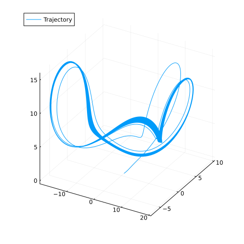
../_images/860195eeefffd341fa7dd2ec250bf4e08550ad15dd8a17953a69ebd3e0851ac1.png

Second-order ODE systems#

ode_order_lowering(sys) automatically transforms a second-order ODE into two first-order ODEs.

using Plots
using ModelingToolkit
using OrdinaryDiffEq

@parameters σ ρ β
@independent_variables t
@variables x(t) y(t) z(t)
D = Differential(t)

eqs = [
    D(D(x)) ~ σ * (y - x),
    D(y) ~ x * (ρ - z) - y,
    D(z) ~ x * y - β * z
]

@mtkbuild sys = ODESystem(eqs, t)

\[\begin{split} \begin{align} \frac{\mathrm{d} \mathtt{xˍt}\left( t \right)}{\mathrm{d}t} &= \left( - x\left( t \right) + y\left( t \right) \right) \sigma \\ \frac{\mathrm{d} y\left( t \right)}{\mathrm{d}t} &= - y\left( t \right) + x\left( t \right) \left( - z\left( t \right) + \rho \right) \\ \frac{\mathrm{d} z\left( t \right)}{\mathrm{d}t} &= x\left( t \right) y\left( t \right) - z\left( t \right) \beta \\ \frac{\mathrm{d} x\left( t \right)}{\mathrm{d}t} &= \mathtt{xˍt}\left( t \right) \end{align} \end{split}\]

Note that you need to provide the initial condition for x’s derivative (D(x)).

u0 = [
    D(x) => 2.0,
    x => 1.0,
    y => 0.0,
    z => 0.0
]

p = [
    σ => 28.0,
    ρ => 10.0,
    β => 8 / 3
]

tspan = (0.0, 100.0)
prob = ODEProblem(sys, u0, tspan, p, jac=true)
sol = solve(prob)
plot(sol, idxs=(x, y, z), label="Trajectory", size=(500, 500))

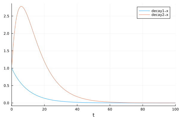
../_images/e79f762d742c3eb104eb621a407bde3de2024cd7aa8d789614d59d4d7545590a.png

Composing systems#

https://docs.sciml.ai/ModelingToolkit/stable/basics/Composition/

By connecting equation(s) to couple ODE systems together, we can build component-based, hierarchical models.

using Plots
using OrdinaryDiffEq
using ModelingToolkit
using ModelingToolkit: t_nounits as t, D_nounits as D

function decay(; name)
    @parameters a
    @variables x(t) f(t)
    ODESystem([
            D(x) ~ -a * x + f
        ], t; name)
end

@named decay1 = decay()
@named decay2 = decay()

WARNING: import of ModelingToolkit.t_nounits into ##415 conflicts with an existing identifier; ignored.
WARNING: import of ModelingToolkit.D_nounits into ##415 conflicts with an existing identifier; ignored.

\[ \begin{align} \frac{\mathrm{d} x\left( t \right)}{\mathrm{d}t} &= f\left( t \right) - a x\left( t \right) \end{align} \]

Define relations (connectors) between the two systems.

connected = compose(
    ODESystem([
            decay2.f ~ decay1.x,
            D(decay1.f) ~ 0], t; name=:connected), decay1, decay2)

equations(connected)

\[\begin{split} \begin{align} \frac{\mathrm{d} \mathtt{decay1.f}\left( t \right)}{\mathrm{d}t} &= 0 \\ \mathtt{decay2.f}\left( t \right) &= \mathtt{decay1.x}\left( t \right) \\ \frac{\mathrm{d} \mathtt{decay1.x}\left( t \right)}{\mathrm{d}t} &= \mathtt{decay1.f}\left( t \right) - \mathtt{decay1.a} \mathtt{decay1.x}\left( t \right) \\ \frac{\mathrm{d} \mathtt{decay2.x}\left( t \right)}{\mathrm{d}t} &= \mathtt{decay2.f}\left( t \right) - \mathtt{decay2.a} \mathtt{decay2.x}\left( t \right) \end{align} \end{split}\]

simplified_sys = structural_simplify(connected)
equations(simplified_sys)

\[\begin{split} \begin{align} \frac{\mathrm{d} \mathtt{decay1.f}\left( t \right)}{\mathrm{d}t} &= -0 \\ \frac{\mathrm{d} \mathtt{decay1.x}\left( t \right)}{\mathrm{d}t} &= \mathtt{decay1.f}\left( t \right) - \mathtt{decay1.a} \mathtt{decay1.x}\left( t \right) \\ \frac{\mathrm{d} \mathtt{decay2.x}\left( t \right)}{\mathrm{d}t} &= \mathtt{decay2.f}\left( t \right) - \mathtt{decay2.a} \mathtt{decay2.x}\left( t \right) \end{align} \end{split}\]

x0 = [decay1.x => 1.0
      decay1.f => 0.0
      decay2.x => 1.0]
p = [decay1.a => 0.1
     decay2.a => 0.2]


tspan = (0.0, 100.0)
sol = solve(ODEProblem(simplified_sys, x0, tspan, p))
plot(sol, idxs=[decay1.x, decay2.x])

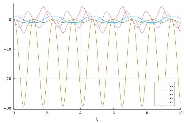
../_images/9605731f73821e99a0f4e0637144c3dad5a68e1c05f41a6bb86bda4ed5b16db2.png

Convert existing functions into MTK systems#

modelingtoolkitize(prob) generates MKT systems from regular DE problems. I t can also generate analytic Jacobin functions for faster solving.

Example: DAE index reduction for the pendulum problem, which cannot be solved by regular ODE solvers.

using Plots
using ModelingToolkit
using OrdinaryDiffEq
using LinearAlgebra

function pendulum!(du, u, p, t)
    x, dx, y, dy, T = u
    g, L = p
    du[1] = dx
    du[2] = T * x
    du[3] = dy
    du[4] = T * y - g
    # Do not write your function like this after you've learned MTK
    du[5] = x^2 + y^2 - L^2
    return nothing
end

pendulum_fun! = ODEFunction(pendulum!, mass_matrix=Diagonal([1, 1, 1, 1, 0]))
u0 = [1.0, 0.0, 0.0, 0.0, 0.0]
p = [9.8, 1.0]
tspan = (0.0, 10.0)
pendulum_prob = ODEProblem(pendulum_fun!, u0, tspan, p)

ODEProblem with uType Vector{Float64} and tType Float64. In-place: true
Non-trivial mass matrix: true
timespan: (0.0, 10.0)
u0: 5-element Vector{Float64}:
 1.0
 0.0
 0.0
 0.0
 0.0

Convert the ODE problem into a MTK system.

tracedSys = modelingtoolkitize(pendulum_prob)

\[\begin{split} \begin{align} \frac{\mathrm{d} \mathtt{x_1}\left( t \right)}{\mathrm{d}t} &= \mathtt{x_2}\left( t \right) \\ \frac{\mathrm{d} \mathtt{x_2}\left( t \right)}{\mathrm{d}t} &= \mathtt{x_1}\left( t \right) \mathtt{x_5}\left( t \right) \\ \frac{\mathrm{d} \mathtt{x_3}\left( t \right)}{\mathrm{d}t} &= \mathtt{x_4}\left( t \right) \\ \frac{\mathrm{d} \mathtt{x_4}\left( t \right)}{\mathrm{d}t} &= - \mathtt{\alpha_1} + \mathtt{x_3}\left( t \right) \mathtt{x_5}\left( t \right) \\ 0 &= \left( \mathtt{x_1}\left( t \right) \right)^{2} + \left( \mathtt{x_3}\left( t \right) \right)^{2} - \mathtt{\alpha_2}^{2} \end{align} \end{split}\]

structural_simplify() and dae_index_lowering() transform the index-3 DAE into an index-0 ODE.

pendulumSys = tracedSys |> dae_index_lowering |> structural_simplify

\[\begin{split} \begin{align} \frac{\mathrm{d} \mathtt{x_1}\left( t \right)}{\mathrm{d}t} &= \mathtt{x_2}\left( t \right) \\ \frac{\mathrm{d} \mathtt{x_2}\left( t \right)}{\mathrm{d}t} &= \mathtt{x_1}\left( t \right) \mathtt{x_5}\left( t \right) \\ \frac{\mathrm{d} \mathtt{x_4}\left( t \right)}{\mathrm{d}t} &= - \mathtt{\alpha_1} + \mathtt{x_3}\left( t \right) \mathtt{x_5}\left( t \right) \\ 0 &= 2 \left( \mathtt{x_4}\left( t \right) \right)^{2} + 2 \left( \mathtt{x_2}\left( t \right) \right)^{2} + 2 \left( \mathtt{x_1}\left( t \right) \right)^{2} \mathtt{x_5}\left( t \right) + 2 \mathtt{x_3}\left( t \right) \left( - \mathtt{\alpha_1} + \mathtt{x_3}\left( t \right) \mathtt{x_5}\left( t \right) \right) \\ 0 &= 2 \mathtt{x_4}\left( t \right) \mathtt{x_3}\left( t \right) + 2 \mathtt{x_1}\left( t \right) \mathtt{x_2}\left( t \right) \end{align} \end{split}\]

The default u0 is included in the system already so one can use an empty array [] as the initial conditions.

prob = ODEProblem(pendulumSys, [], tspan);
sol = solve(prob, Rodas5P(), abstol=1e-8, reltol=1e-8)

┌ Warning: Initialization system is overdetermined. 2 equations for 0 unknowns. Initialization will default to using least squares. `SCCNonlinearProblem` can only be used for initialization of fully determined systems and hence will not be used here. To suppress this warning pass warn_initialize_determined = false. To make this warning into an error, pass fully_determined = true
└ @ ModelingToolkit ~/.julia/packages/ModelingToolkit/EpUEk/src/systems/diffeqs/abstractodesystem.jl:1522

retcode: Success
Interpolation: specialized 4rd order "free" stiffness-aware interpolation
t: 5885-element Vector{Float64}:
  0.0
  8.820490580568942e-7
  1.1305014555891484e-6
  1.3789538531214025e-6
  1.6915316787116988e-6
  2.1502965001609697e-6
  2.8783820404427622e-6
  3.896377133997462e-6
  5.347182593843697e-6
  7.050721914091127e-6
  ⋮
  9.974867778864727
  9.978567737582472
  9.981896651586998
  9.985225565591525
  9.988554479596052
  9.99188339360058
  9.995212307605106
  9.998541221609633
 10.0
u: 5885-element Vector{Vector{Float64}}:
 [1.0, 0.0, 0.0, 0.0, 0.0]
 [1.0, 3.199780977062103e-15, -8.644080768957695e-6, 2.3539169203643222e-8, 2.4095805444881106e-9]
 [1.0, 2.7482280349864486e-15, -1.1078914264773797e-5, -1.8191090934184693e-9, -1.730986481767613e-10]
 [1.0, 3.483841782799009e-15, -1.3513747760589899e-5, 2.67635632067077e-9, 2.9173241828649165e-10]
 [1.0, 4.1771062187710175e-15, -1.657701045137486e-5, 2.164490120014696e-9, 2.489068770938456e-10]
 [1.0, 5.131322600755049e-15, -2.1072905701577752e-5, 1.947239983997743e-9, 2.440109529291154e-10]
 [1.0, 6.360308038900883e-15, -2.8208143996339387e-5, 1.4091837776807127e-9, 2.2498807810193164e-10]
 [1.0, 7.318479526291965e-15, -3.818449591317555e-5, 4.163792911809305e-10, 1.912688795228826e-10]
 [1.0, 6.591838516098067e-15, -5.240238941966877e-5, -1.5270066361242033e-9, 1.243881408945314e-10]
 [1.0, 1.539896768006486e-15, -6.90970747580938e-5, -4.562445483185924e-9, 2.1628597646905967e-11]
 ⋮
 [0.397242108666797, -3.892145279280729, -1.684753693270005, -26.980733671710855, -0.9177151554797046]
 [0.3827686965430455, -3.9312097549103058, -1.6287831878887693, -27.160965630867018, -0.923845508997523]
 [0.3696249808157838, -3.965323220548635, -1.577389599804099, -27.317867322140128, -0.9291823143511242]
 [0.3563693777433982, -3.9984262863493703, -1.525041065220585, -27.46969219483144, -0.9343464380970998]
 [0.3430053003830553, -4.030489317561693, -1.4717641453861465, -27.616348073251665, -0.9393347452988721]
 [0.32953625923436153, -4.0614834135616364, -1.4175864906197515, -27.757745440706028, -0.9441441911667372]
 [0.31596585971898045, -4.091380453707269, -1.3625368168572172, -27.89379753895679, -0.9487718247374346]
 [0.30229779950894203, -4.120153142371051, -1.3066448800464476, -28.024420471269615, -0.9532147923796632]
 [0.2962784489477445, -4.132400642008936, -1.2818946506820865, -28.07992961918143, -0.9551028643231755]

plot(sol, idxs=unknowns(tracedSys))

../_images/639384b0a1b4b1f6bff1367b57892c452fa2edfea5767be5332ff5383e391c7d.png

This notebook was generated using Literate.jl.