Ordinary Differential Equations (ODEs)

Ordinary Differential Equations (ODEs)#

DifferentialEquations.jl docs

Define a model function representing the right-hand-side (RHS) of the system.

Out-of-place form: f(u, p, t) where u is the state variable(s), p is the parameter(s), and t is the independent variable (usually time). The output is the right hand side (RHS) of the differential equation system.
In-place form: f!(du, u, p, t), where the output is saved to du. The rest is the same as the out-of-place form. The in-place function may be faster since it does not allocate a new array in each call.
Initial conditions (u0) for the state variable(s).
(Optional) parameter(s) p.
Define a problem (e.g. ODEProblem) using the model function (f), initial condition(s) (u0), simulation time span (tspan == (tstart, tend)), and parameter(s) p.
Solve the problem by calling solve(prob).

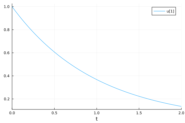
Radioactive decay example#

The decaying rate of a nuclear isotope is proportional to its concentration (number):

\[ \frac{d}{dt}C(t) = - \lambda C(t) \]

State variable(s)

\(C(t)\): The concentration (number) of a decaying nuclear isotope.

Parameter(s)

\(\lambda\): The rate constant of nuclear decay. The half-life: \(t_{\frac{1}{2}} = \frac{ln2}{\lambda}\).

using OrdinaryDiffEq
using Plots

The exponential decay ODE model, out-of-place (3-parameter) form

expdecay(u, p, t) = p * u

expdecay (generic function with 1 method)

Setup ODE problem

p = -1.0 ## Parameter
u0 = 1.0 ## Initial condition
tspan = (0.0, 2.0) ## Simulation start and end time points
prob = ODEProblem(expdecay, u0, tspan, p) ## Define the problem
sol = solve(prob) ## Solve the problem

retcode: Success
Interpolation: 3rd order Hermite
t: 8-element Vector{Float64}:
0
10001999200479662
34208427066999536
6553980136343391
0312652525315806
4709405856363595
9659576669700232
0
u: 8-element Vector{Float64}:
0
9048193287657775
7102883621328676
5192354400036404
35655576576996556
2297097907863828
14002247272452764
1353360028400881

Visualize the solution with Plots.jl.

plot(sol)

../_images/f6902fac41d0ad035b67bab4bcd652f1526889e253f77a10cd57608d85be5947.png

Solution handling#

https://docs.sciml.ai/DiffEqDocs/stable/basics/solution/ The mostly used feature is sol(t), the state variables at time t. t could be a scalar or a vector-like sequence. The result state variables are calculated with interpolation.

sol(1.0)

0.3678796381978344

sol(0.0:0.1:2.0)

t: 0.0:0.1:2.0
u: 21-element Vector{Float64}:
0
9048374180989603
8187305973051514
7408182261974484
670319782243577
6065302341562359
5488116548085096
49658509875978446
4493280239179766
4065692349272286
 ⋮
30119273799114377
2725309051375336
24659717503493142
22313045099430742
20189530933816474
18268185222253558
16529821250790575
14956912660454402
13533600284008812

sol.t: time points by the solver.

sol.t

8-element Vector{Float64}:
0
10001999200479662
34208427066999536
6553980136343391
0312652525315806
4709405856363595
9659576669700232
0

sol.u: state variables at sol.t.

sol.u

8-element Vector{Float64}:
0
9048193287657775
7102883621328676
5192354400036404
35655576576996556
2297097907863828
14002247272452764
1353360028400881

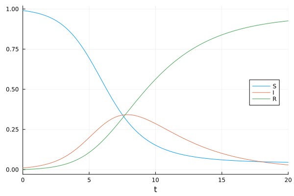
The SIR model#

A more complicated example is the SIR model describing infectious disease spreading. There are 3 state variables and 2 parameters.

\[\begin{split} \begin{align} \frac{d}{dt}S(t) &= - \beta S(t)I(t) \\ \frac{d}{dt}I(t) &= \beta S(t)I(t) - \gamma I(t) \\ \frac{d}{dt}R(t) &= \gamma I(t) \end{align} \end{split}\]

State variable(s)

\(S(t)\) : the fraction of susceptible people
\(I(t)\) : the fraction of infectious people
\(R(t)\) : the fraction of recovered (or removed) people

Parameter(s)

\(\beta\) : the rate of infection when susceptible and infectious people meet
\(\gamma\) : the rate of recovery of infectious people

using OrdinaryDiffEq
using Plots

Here we use the in-place form: f!(du, u, p ,t) for the SIR model. The output is written to the first argument du, without allocating a new array in each function call.

function sir!(du, u, p, t)
    s, i, r = u
    β, γ = p
    v1 = β * s * i
    v2 = γ * i
    du[1] = -v1
    du[2] = v1 - v2
    du[3] = v2
    return nothing
end

sir! (generic function with 1 method)

Setup parameters, initial conditions, time span, and the ODE problem.

p = (β=1.0, γ=0.3)
u0 = [0.99, 0.01, 0.00]
tspan = (0.0, 20.0)
prob = ODEProblem(sir!, u0, tspan, p)

ODEProblem with uType Vector{Float64} and tType Float64. In-place: true
Non-trivial mass matrix: false
timespan: (0.0, 20.0)
u0: 3-element Vector{Float64}:
 0.99
 0.01
 0.0

Solve the problem

sol = solve(prob)

retcode: Success
Interpolation: 3rd order Hermite
t: 17-element Vector{Float64}:
  0.0
  0.08921318693905476
  0.3702862715172094
  0.7984257132319627
  1.3237271485666187
  1.991841832691831
  2.7923706947355837
  3.754781614278828
  4.901904318934307
  6.260476636498209
  7.7648912410433075
  9.39040980993922
 11.483861023017885
 13.372369854616487
 15.961357172044833
 18.681426667664056
 20.0
u: 17-element Vector{Vector{Float64}}:
 [0.99, 0.01, 0.0]
 [0.9890894703413342, 0.010634484617786016, 0.00027604504087978485]
 [0.9858331594901347, 0.012901496825852227, 0.0012653436840130785]
 [0.9795270529591532, 0.017282420996456258, 0.003190526044390597]
 [0.9689082167415561, 0.02463126703444545, 0.006460516223998508]
 [0.9490552312363142, 0.03827338797605378, 0.012671380787632141]
 [0.9118629475333939, 0.06347250098224964, 0.024664551484356558]
 [0.8398871089274511, 0.11078176031568547, 0.049331130756863524]
 [0.7075842068024722, 0.19166147882272844, 0.1007543143747994]
 [0.508146028721987, 0.29177419341470584, 0.20007977786330722]
 [0.31213222024413995, 0.3415879120018046, 0.34627986775405545]
 [0.18215683096365565, 0.3099983134156389, 0.5078448556207055]
 [0.10427205468919205, 0.22061114011133276, 0.6751168051994751]
 [0.07386737407725845, 0.14760143051851143, 0.7785311954042301]
 [0.05545028910907714, 0.07997076922865315, 0.8645789416622697]
 [0.047334990695892025, 0.04060565321383335, 0.9120593560902746]
 [0.04522885458929332, 0.029057416110814603, 0.925713729299892]

Visualize the solution

plot(sol, labels=["S" "I" "R"], legend=:right)

../_images/31b518e413cfef1b0c654701a189e326b562f4f525fbf08f2a6ff4360fe974fd.png

sol[i]: all components at time step i

sol[2]

3-element Vector{Float64}:
9890894703413342
010634484617786016
00027604504087978485

sol[i, j]: ith component at time step j

sol[1, 2]

0.9890894703413342

sol[i, :]: the time series for the ith component.

sol[1, :]

17-element Vector{Float64}:
99
9890894703413342
9858331594901347
9795270529591532
9689082167415561
9490552312363142
9118629475333939
8398871089274511
7075842068024722
508146028721987
31213222024413995
18215683096365565
10427205468919205
07386737407725845
05545028910907714
047334990695892025
04522885458929332

sol(t, idxs=1): the 1st element in time point(s) t with interpolation. t can be a scalar or a vector.

sol(10, idxs=2)

0.28576194586813003

sol(0.0:0.1:20.0, idxs=2)

t: 0.0:0.1:20.0
u: 201-element Vector{Float64}:
01
010713819530291442
01147737632963402
012293955863322855
013167034902663112
014100286700885235
015097588761311391
016163031360643162
01730091874845442
018515771780096318
 ⋮
03561030823283819
03471833422630802
03384816241692694
03299928861769087
032171218254199684
031363466364657075
030575557599870556
029807026223251362
029057416110814645

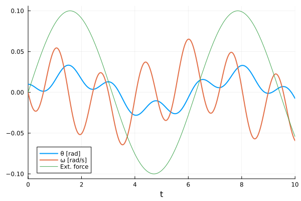
Non-autonomous ODEs#

In non-autonomous ODEs, term(s) in the right-hand-side (RHS) maybe time-dependent. For example, in this pendulum model has an external, time-dependent, force.

\[\begin{split} \begin{aligned} \dot{\theta} &= \omega(t) \\ \dot{\omega} &= -1.5\frac{g}{l}sin(\theta(t)) + \frac{3}{ml^2}M(t) \end{aligned} \end{split}\]

\(\theta\): pendulum angle
\(\omega\): angular rate
M: time-dependent external torque
\(l\): pendulum length
\(g\): gradational acceleration

using OrdinaryDiffEq
using Plots

function pendulum!(du, u, p, t)
    l = 1.0                             ## length [m]
    m = 1.0                             ## mass [kg]
    g = 9.81                            ## gravitational acceleration [m/s²]
    du[1] = u[2]                        ## θ'(t) = ω(t)
    du[2] = -3g / (2l) * sin(u[1]) + 3 / (m * l^2) * p(t) # ω'(t) = -3g/(2l) sin θ(t) + 3/(ml^2)M(t)
    return nothing
end

u0 = [0.01, 0.0]                     ## initial angular deflection [rad] and angular velocity [rad/s]
tspan = (0.0, 10.0)                  ## time interval

M = t -> 0.1 * sin(t)                   ## external torque [Nm] as the parameter for the pendulum model

prob = ODEProblem(pendulum!, u0, tspan, M)
sol = solve(prob)

plot(sol, linewidth=2, xaxis="t", label=["θ [rad]" "ω [rad/s]"])
plot!(M, tspan..., label="Ext. force")

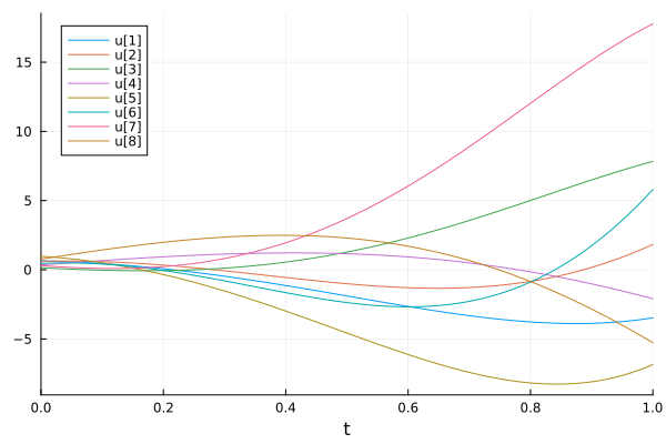
../_images/b70a9fe5fddc4946f6519a2f823149a21b4dba89b50e2e5d5ba7be9e0c9b88bb.png

Linear ODE system#

The ODE system could be anything as long as it returns the derivatives of state variables. In this example, the ODE system is described by a matrix differential operator.

\(\dot{u} = Au\)

using OrdinaryDiffEq
using Plots

A = [
    1.0 0 0 -5
    4 -2 4 -3
    -4 0 0 1
    5 -2 2 3
]

u0 = rand(4, 2)

tspan = (0.0, 1.0)
f = (u, p, t) -> A * u
prob = ODEProblem(f, u0, tspan)
sol = solve(prob)
plot(sol)

../_images/ea61ffc7c7bd4fc4d5ff4d687b57598a464d156e95531d94e1adb7dacaacf5da.png

This notebook was generated using Literate.jl.