Symbolic calculations in Julia

Symbolic calculations in Julia#

Symbolics.jl is a computer Algebra System (CAS) for Julia. The symbols are number-like and follow Julia semantics so we can put them into a regular function to get a symbolic counterpart. Symbolics.jl is the backbone of ModelingToolkit.jl. Comparision to SymPy

Source:

Simulating Big Models in Julia with ModelingToolkit @ JuliaCon 2021 Workshop.
Symbolics.jl Github repo and its docs.

Caveats about Symbolics.jl#

Symbolics.jl can only handle traceble, quasi-static expressions. However, some expressions are not quasi-static e.g. factorial. The number of operations depends on the input value.

Use @register_symbolic to stop Symbolics.jl from digging further.

Some code paths is untraceable, such as conditional statements: if…else…end.

You can use ifelse(cond, ex1, ex2) or (cond) * (ex1) + (1 - cond) * (ex2) to make it traceable.

Basic operations#

latexify
derivative
gradient
jacobian
substitute
simplify

using Symbolics
using Latexify

@variables x y
x^2 + y^2

\[ \begin{equation} x^{2} + y^{2} \end{equation} \]

You can use Latexify.latexify() to see the LaTeX code.

A = [
    x^2+y 0 2x
    0 0 2y
    y^2+x 0 0
]

latexify(A)

\[\begin{split}\begin{equation} \left[ \begin{array}{ccc} y + x^{2} & 0 & 2 x \\ 0 & 0 & 2 y \\ x + y^{2} & 0 & 0 \\ \end{array} \right] \end{equation}\end{split}\]

Derivative: Symbolics.derivative(expr, variable)

Symbolics.derivative(x^2 + y^2, x)

\[ \begin{equation} 2 x \end{equation} \]

Gradient: Symbolics.gradient(expr, [variables])

Symbolics.gradient(x^2 + y^2, [x, y])

\[\begin{split} \begin{equation} \left[ \begin{array}{c} 2 x \\ 2 y \\ \end{array} \right] \end{equation} \end{split}\]

Jacobian: Symbolics.jacobian([exprs], [variables])

Symbolics.jacobian([x^2 + y^2; y^2], [x, y])

\[\begin{split} \begin{equation} \left[ \begin{array}{cc} 2 x & 2 y \\ 0 & 2 y \\ \end{array} \right] \end{equation} \end{split}\]

Substitute: Symbolics.substitute(expr, mapping)

Symbolics.substitute(sin(x)^2 + 2 + cos(x)^2, Dict(x => y^2))

\[ \begin{equation} 2 + \sin^{2}\left( y^{2} \right) + \cos^{2}\left( y^{2} \right) \end{equation} \]

Symbolics.substitute(sin(x)^2 + 2 + cos(x)^2, Dict(x => 1.0))

\[ \begin{equation} 3 \end{equation} \]

Simplify: Symbolics.simplify(expr)

Symbolics.simplify(sin(x)^2 + 2 + cos(x)^2)

\[ \begin{equation} 3 \end{equation} \]

This expression gets automatically simplified because it’s always true

2x - x

\[ \begin{equation} x \end{equation} \]

ex = x^2 + y^2 + sin(x)
isequal(2ex, ex + ex)

false

You need to simplify the expressions.

isequal(simplify(2ex), simplify(ex + ex))

true

ex / ex

\[ \begin{equation} 1 \end{equation} \]

Symbolic integration: use SymbolicNumericIntegration.jl. The Youtube video by doggo dot jl gives a concise example.

Custom functions#

https://docs.sciml.ai/Symbolics/stable/manual/functions/

With @register_symbolic and @register_array_symbolic, functions will be evaluated as-is and will not be traced and expanded by Symbolics.jl. Useful for rand(), data interpolations, etc.

More number types#

Complex number

@variables z::Complex

\[\begin{split} \begin{equation} \left[ \begin{array}{c} \mathrm{real}\left( z \right) + \mathrm{imag}\left( z \right) \mathit{i} \\ \end{array} \right] \end{equation} \end{split}\]

Array types with subscript

@variables xs[1:20]

1-element Vector{Symbolics.Arr{Symbolics.Num, 1}}:
 xs[1:20]

xs[1]

\[ \begin{equation} \mathtt{xs}_{1} \end{equation} \]

Explicit vector form

collect(xs)

\[\begin{split} \begin{equation} \left[ \begin{array}{c} \mathtt{xs}_{1} \\ \mathtt{xs}_{2} \\ \mathtt{xs}_{3} \\ \mathtt{xs}_{4} \\ \mathtt{xs}_{5} \\ \mathtt{xs}_{6} \\ \mathtt{xs}_{7} \\ \mathtt{xs}_{8} \\ \mathtt{xs}_{9} \\ \mathtt{xs}_{10} \\ \mathtt{xs}_{11} \\ \mathtt{xs}_{12} \\ \mathtt{xs}_{13} \\ \mathtt{xs}_{14} \\ \mathtt{xs}_{15} \\ \mathtt{xs}_{16} \\ \mathtt{xs}_{17} \\ \mathtt{xs}_{18} \\ \mathtt{xs}_{19} \\ \mathtt{xs}_{20} \\ \end{array} \right] \end{equation} \end{split}\]

Operations on arrays are supported

sum(collect(xs))

\[ \begin{equation} \mathtt{xs}_{1} + \mathtt{xs}_{10} + \mathtt{xs}_{11} + \mathtt{xs}_{12} + \mathtt{xs}_{13} + \mathtt{xs}_{14} + \mathtt{xs}_{15} + \mathtt{xs}_{16} + \mathtt{xs}_{17} + \mathtt{xs}_{18} + \mathtt{xs}_{19} + \mathtt{xs}_{2} + \mathtt{xs}_{20} + \mathtt{xs}_{3} + \mathtt{xs}_{4} + \mathtt{xs}_{5} + \mathtt{xs}_{6} + \mathtt{xs}_{7} + \mathtt{xs}_{8} + \mathtt{xs}_{9} \end{equation} \]

Example: Rosenbrock function#

Wikipedia: https://en.wikipedia.org/wiki/Rosenbrock_function

We use the vector form of Rosenbrock function.

rosenbrock(xs) = sum(1:length(xs)-1) do i
    100 * (xs[i+1] - xs[i]^2)^2 + (1 - xs[i])^2
end

rosenbrock (generic function with 1 method)

The function is at minimum when xs are all one’s

rosenbrock(ones(100))

0.0

Making a 20-element array

N = 20
@variables xs[1:N]

1-element Vector{Symbolics.Arr{Symbolics.Num, 1}}:
 xs[1:20]

A full list of vector components

xs = collect(xs)

\[\begin{split} \begin{equation} \left[ \begin{array}{c} \mathtt{xs}_{1} \\ \mathtt{xs}_{2} \\ \mathtt{xs}_{3} \\ \mathtt{xs}_{4} \\ \mathtt{xs}_{5} \\ \mathtt{xs}_{6} \\ \mathtt{xs}_{7} \\ \mathtt{xs}_{8} \\ \mathtt{xs}_{9} \\ \mathtt{xs}_{10} \\ \mathtt{xs}_{11} \\ \mathtt{xs}_{12} \\ \mathtt{xs}_{13} \\ \mathtt{xs}_{14} \\ \mathtt{xs}_{15} \\ \mathtt{xs}_{16} \\ \mathtt{xs}_{17} \\ \mathtt{xs}_{18} \\ \mathtt{xs}_{19} \\ \mathtt{xs}_{20} \\ \end{array} \right] \end{equation} \end{split}\]

rxs = rosenbrock(xs)

\[ \begin{equation} \left( 1 - \mathtt{xs}_{1} \right)^{2} + \left( 1 - \mathtt{xs}_{10} \right)^{2} + \left( 1 - \mathtt{xs}_{11} \right)^{2} + \left( 1 - \mathtt{xs}_{12} \right)^{2} + \left( 1 - \mathtt{xs}_{13} \right)^{2} + \left( 1 - \mathtt{xs}_{14} \right)^{2} + \left( 1 - \mathtt{xs}_{15} \right)^{2} + \left( 1 - \mathtt{xs}_{16} \right)^{2} + \left( 1 - \mathtt{xs}_{17} \right)^{2} + \left( 1 - \mathtt{xs}_{18} \right)^{2} + \left( 1 - \mathtt{xs}_{19} \right)^{2} + \left( 1 - \mathtt{xs}_{2} \right)^{2} + \left( 1 - \mathtt{xs}_{3} \right)^{2} + \left( 1 - \mathtt{xs}_{4} \right)^{2} + \left( 1 - \mathtt{xs}_{5} \right)^{2} + \left( 1 - \mathtt{xs}_{6} \right)^{2} + \left( 1 - \mathtt{xs}_{7} \right)^{2} + \left( 1 - \mathtt{xs}_{8} \right)^{2} + \left( 1 - \mathtt{xs}_{9} \right)^{2} + 100 \left( \mathtt{xs}_{2} - \left( \mathtt{xs}_{1} \right)^{2} \right)^{2} + 100 \left( \mathtt{xs}_{11} - \left( \mathtt{xs}_{10} \right)^{2} \right)^{2} + 100 \left( \mathtt{xs}_{12} - \left( \mathtt{xs}_{11} \right)^{2} \right)^{2} + 100 \left( \mathtt{xs}_{13} - \left( \mathtt{xs}_{12} \right)^{2} \right)^{2} + 100 \left( \mathtt{xs}_{14} - \left( \mathtt{xs}_{13} \right)^{2} \right)^{2} + 100 \left( \mathtt{xs}_{15} - \left( \mathtt{xs}_{14} \right)^{2} \right)^{2} + 100 \left( \mathtt{xs}_{16} - \left( \mathtt{xs}_{15} \right)^{2} \right)^{2} + 100 \left( \mathtt{xs}_{17} - \left( \mathtt{xs}_{16} \right)^{2} \right)^{2} + 100 \left( \mathtt{xs}_{18} - \left( \mathtt{xs}_{17} \right)^{2} \right)^{2} + 100 \left( \mathtt{xs}_{19} - \left( \mathtt{xs}_{18} \right)^{2} \right)^{2} + 100 \left( \mathtt{xs}_{20} - \left( \mathtt{xs}_{19} \right)^{2} \right)^{2} + 100 \left( \mathtt{xs}_{3} - \left( \mathtt{xs}_{2} \right)^{2} \right)^{2} + 100 \left( \mathtt{xs}_{4} - \left( \mathtt{xs}_{3} \right)^{2} \right)^{2} + 100 \left( \mathtt{xs}_{5} - \left( \mathtt{xs}_{4} \right)^{2} \right)^{2} + 100 \left( \mathtt{xs}_{6} - \left( \mathtt{xs}_{5} \right)^{2} \right)^{2} + 100 \left( \mathtt{xs}_{7} - \left( \mathtt{xs}_{6} \right)^{2} \right)^{2} + 100 \left( \mathtt{xs}_{8} - \left( \mathtt{xs}_{7} \right)^{2} \right)^{2} + 100 \left( \mathtt{xs}_{9} - \left( \mathtt{xs}_{8} \right)^{2} \right)^{2} + 100 \left( \mathtt{xs}_{10} - \left( \mathtt{xs}_{9} \right)^{2} \right)^{2} \end{equation} \]

Gradient

grad = Symbolics.gradient(rxs, xs)

\[\begin{split} \begin{equation} \left[ \begin{array}{c} - 2 \left( 1 - \mathtt{xs}_{1} \right) - 400 \mathtt{xs}_{1} \left( \mathtt{xs}_{2} - \left( \mathtt{xs}_{1} \right)^{2} \right) \\ - 2 \left( 1 - \mathtt{xs}_{2} \right) + 200 \left( \mathtt{xs}_{2} - \left( \mathtt{xs}_{1} \right)^{2} \right) - 400 \mathtt{xs}_{2} \left( \mathtt{xs}_{3} - \left( \mathtt{xs}_{2} \right)^{2} \right) \\ - 2 \left( 1 - \mathtt{xs}_{3} \right) + 200 \left( \mathtt{xs}_{3} - \left( \mathtt{xs}_{2} \right)^{2} \right) - 400 \mathtt{xs}_{3} \left( \mathtt{xs}_{4} - \left( \mathtt{xs}_{3} \right)^{2} \right) \\ - 2 \left( 1 - \mathtt{xs}_{4} \right) + 200 \left( \mathtt{xs}_{4} - \left( \mathtt{xs}_{3} \right)^{2} \right) - 400 \mathtt{xs}_{4} \left( \mathtt{xs}_{5} - \left( \mathtt{xs}_{4} \right)^{2} \right) \\ - 2 \left( 1 - \mathtt{xs}_{5} \right) + 200 \left( \mathtt{xs}_{5} - \left( \mathtt{xs}_{4} \right)^{2} \right) - 400 \mathtt{xs}_{5} \left( \mathtt{xs}_{6} - \left( \mathtt{xs}_{5} \right)^{2} \right) \\ - 2 \left( 1 - \mathtt{xs}_{6} \right) + 200 \left( \mathtt{xs}_{6} - \left( \mathtt{xs}_{5} \right)^{2} \right) - 400 \mathtt{xs}_{6} \left( \mathtt{xs}_{7} - \left( \mathtt{xs}_{6} \right)^{2} \right) \\ - 2 \left( 1 - \mathtt{xs}_{7} \right) + 200 \left( \mathtt{xs}_{7} - \left( \mathtt{xs}_{6} \right)^{2} \right) - 400 \mathtt{xs}_{7} \left( \mathtt{xs}_{8} - \left( \mathtt{xs}_{7} \right)^{2} \right) \\ - 2 \left( 1 - \mathtt{xs}_{8} \right) + 200 \left( \mathtt{xs}_{8} - \left( \mathtt{xs}_{7} \right)^{2} \right) - 400 \mathtt{xs}_{8} \left( \mathtt{xs}_{9} - \left( \mathtt{xs}_{8} \right)^{2} \right) \\ - 2 \left( 1 - \mathtt{xs}_{9} \right) + 200 \left( \mathtt{xs}_{9} - \left( \mathtt{xs}_{8} \right)^{2} \right) - 400 \mathtt{xs}_{9} \left( \mathtt{xs}_{10} - \left( \mathtt{xs}_{9} \right)^{2} \right) \\ - 2 \left( 1 - \mathtt{xs}_{10} \right) + 200 \left( \mathtt{xs}_{10} - \left( \mathtt{xs}_{9} \right)^{2} \right) - 400 \mathtt{xs}_{10} \left( \mathtt{xs}_{11} - \left( \mathtt{xs}_{10} \right)^{2} \right) \\ - 2 \left( 1 - \mathtt{xs}_{11} \right) + 200 \left( \mathtt{xs}_{11} - \left( \mathtt{xs}_{10} \right)^{2} \right) - 400 \mathtt{xs}_{11} \left( \mathtt{xs}_{12} - \left( \mathtt{xs}_{11} \right)^{2} \right) \\ - 2 \left( 1 - \mathtt{xs}_{12} \right) + 200 \left( \mathtt{xs}_{12} - \left( \mathtt{xs}_{11} \right)^{2} \right) - 400 \mathtt{xs}_{12} \left( \mathtt{xs}_{13} - \left( \mathtt{xs}_{12} \right)^{2} \right) \\ - 2 \left( 1 - \mathtt{xs}_{13} \right) + 200 \left( \mathtt{xs}_{13} - \left( \mathtt{xs}_{12} \right)^{2} \right) - 400 \mathtt{xs}_{13} \left( \mathtt{xs}_{14} - \left( \mathtt{xs}_{13} \right)^{2} \right) \\ - 2 \left( 1 - \mathtt{xs}_{14} \right) + 200 \left( \mathtt{xs}_{14} - \left( \mathtt{xs}_{13} \right)^{2} \right) - 400 \mathtt{xs}_{14} \left( \mathtt{xs}_{15} - \left( \mathtt{xs}_{14} \right)^{2} \right) \\ - 2 \left( 1 - \mathtt{xs}_{15} \right) + 200 \left( \mathtt{xs}_{15} - \left( \mathtt{xs}_{14} \right)^{2} \right) - 400 \mathtt{xs}_{15} \left( \mathtt{xs}_{16} - \left( \mathtt{xs}_{15} \right)^{2} \right) \\ - 2 \left( 1 - \mathtt{xs}_{16} \right) + 200 \left( \mathtt{xs}_{16} - \left( \mathtt{xs}_{15} \right)^{2} \right) - 400 \mathtt{xs}_{16} \left( \mathtt{xs}_{17} - \left( \mathtt{xs}_{16} \right)^{2} \right) \\ - 2 \left( 1 - \mathtt{xs}_{17} \right) + 200 \left( \mathtt{xs}_{17} - \left( \mathtt{xs}_{16} \right)^{2} \right) - 400 \mathtt{xs}_{17} \left( \mathtt{xs}_{18} - \left( \mathtt{xs}_{17} \right)^{2} \right) \\ - 2 \left( 1 - \mathtt{xs}_{18} \right) + 200 \left( \mathtt{xs}_{18} - \left( \mathtt{xs}_{17} \right)^{2} \right) - 400 \mathtt{xs}_{18} \left( \mathtt{xs}_{19} - \left( \mathtt{xs}_{18} \right)^{2} \right) \\ - 2 \left( 1 - \mathtt{xs}_{19} \right) + 200 \left( \mathtt{xs}_{19} - \left( \mathtt{xs}_{18} \right)^{2} \right) - 400 \mathtt{xs}_{19} \left( \mathtt{xs}_{20} - \left( \mathtt{xs}_{19} \right)^{2} \right) \\ 200 \left( \mathtt{xs}_{20} - \left( \mathtt{xs}_{19} \right)^{2} \right) \\ \end{array} \right] \end{equation} \end{split}\]

Hessian = Jacobian of gradient

hes1 = Symbolics.jacobian(grad, xs)

\[\begin{split} \begin{equation} \left[ \begin{array}{cccccccccccccccccccc} 2 + 800 \left( \mathtt{xs}_{1} \right)^{2} - 400 \left( \mathtt{xs}_{2} - \left( \mathtt{xs}_{1} \right)^{2} \right) & - 400 \mathtt{xs}_{1} & 0 & 0 & 0 & 0 & 0 & 0 & 0 & 0 & 0 & 0 & 0 & 0 & 0 & 0 & 0 & 0 & 0 & 0 \\ - 400 \mathtt{xs}_{1} & 202 - 400 \left( \mathtt{xs}_{3} - \left( \mathtt{xs}_{2} \right)^{2} \right) + 800 \left( \mathtt{xs}_{2} \right)^{2} & - 400 \mathtt{xs}_{2} & 0 & 0 & 0 & 0 & 0 & 0 & 0 & 0 & 0 & 0 & 0 & 0 & 0 & 0 & 0 & 0 & 0 \\ 0 & - 400 \mathtt{xs}_{2} & 202 + 800 \left( \mathtt{xs}_{3} \right)^{2} - 400 \left( \mathtt{xs}_{4} - \left( \mathtt{xs}_{3} \right)^{2} \right) & - 400 \mathtt{xs}_{3} & 0 & 0 & 0 & 0 & 0 & 0 & 0 & 0 & 0 & 0 & 0 & 0 & 0 & 0 & 0 & 0 \\ 0 & 0 & - 400 \mathtt{xs}_{3} & 202 - 400 \left( \mathtt{xs}_{5} - \left( \mathtt{xs}_{4} \right)^{2} \right) + 800 \left( \mathtt{xs}_{4} \right)^{2} & - 400 \mathtt{xs}_{4} & 0 & 0 & 0 & 0 & 0 & 0 & 0 & 0 & 0 & 0 & 0 & 0 & 0 & 0 & 0 \\ 0 & 0 & 0 & - 400 \mathtt{xs}_{4} & 202 + 800 \left( \mathtt{xs}_{5} \right)^{2} - 400 \left( \mathtt{xs}_{6} - \left( \mathtt{xs}_{5} \right)^{2} \right) & - 400 \mathtt{xs}_{5} & 0 & 0 & 0 & 0 & 0 & 0 & 0 & 0 & 0 & 0 & 0 & 0 & 0 & 0 \\ 0 & 0 & 0 & 0 & - 400 \mathtt{xs}_{5} & 202 - 400 \left( \mathtt{xs}_{7} - \left( \mathtt{xs}_{6} \right)^{2} \right) + 800 \left( \mathtt{xs}_{6} \right)^{2} & - 400 \mathtt{xs}_{6} & 0 & 0 & 0 & 0 & 0 & 0 & 0 & 0 & 0 & 0 & 0 & 0 & 0 \\ 0 & 0 & 0 & 0 & 0 & - 400 \mathtt{xs}_{6} & 202 + 800 \left( \mathtt{xs}_{7} \right)^{2} - 400 \left( \mathtt{xs}_{8} - \left( \mathtt{xs}_{7} \right)^{2} \right) & - 400 \mathtt{xs}_{7} & 0 & 0 & 0 & 0 & 0 & 0 & 0 & 0 & 0 & 0 & 0 & 0 \\ 0 & 0 & 0 & 0 & 0 & 0 & - 400 \mathtt{xs}_{7} & 202 + 800 \left( \mathtt{xs}_{8} \right)^{2} - 400 \left( \mathtt{xs}_{9} - \left( \mathtt{xs}_{8} \right)^{2} \right) & - 400 \mathtt{xs}_{8} & 0 & 0 & 0 & 0 & 0 & 0 & 0 & 0 & 0 & 0 & 0 \\ 0 & 0 & 0 & 0 & 0 & 0 & 0 & - 400 \mathtt{xs}_{8} & 202 + 800 \left( \mathtt{xs}_{9} \right)^{2} - 400 \left( \mathtt{xs}_{10} - \left( \mathtt{xs}_{9} \right)^{2} \right) & - 400 \mathtt{xs}_{9} & 0 & 0 & 0 & 0 & 0 & 0 & 0 & 0 & 0 & 0 \\ 0 & 0 & 0 & 0 & 0 & 0 & 0 & 0 & - 400 \mathtt{xs}_{9} & 202 - 400 \left( \mathtt{xs}_{11} - \left( \mathtt{xs}_{10} \right)^{2} \right) + 800 \left( \mathtt{xs}_{10} \right)^{2} & - 400 \mathtt{xs}_{10} & 0 & 0 & 0 & 0 & 0 & 0 & 0 & 0 & 0 \\ 0 & 0 & 0 & 0 & 0 & 0 & 0 & 0 & 0 & - 400 \mathtt{xs}_{10} & 202 + 800 \left( \mathtt{xs}_{11} \right)^{2} - 400 \left( \mathtt{xs}_{12} - \left( \mathtt{xs}_{11} \right)^{2} \right) & - 400 \mathtt{xs}_{11} & 0 & 0 & 0 & 0 & 0 & 0 & 0 & 0 \\ 0 & 0 & 0 & 0 & 0 & 0 & 0 & 0 & 0 & 0 & - 400 \mathtt{xs}_{11} & 202 - 400 \left( \mathtt{xs}_{13} - \left( \mathtt{xs}_{12} \right)^{2} \right) + 800 \left( \mathtt{xs}_{12} \right)^{2} & - 400 \mathtt{xs}_{12} & 0 & 0 & 0 & 0 & 0 & 0 & 0 \\ 0 & 0 & 0 & 0 & 0 & 0 & 0 & 0 & 0 & 0 & 0 & - 400 \mathtt{xs}_{12} & 202 - 400 \left( \mathtt{xs}_{14} - \left( \mathtt{xs}_{13} \right)^{2} \right) + 800 \left( \mathtt{xs}_{13} \right)^{2} & - 400 \mathtt{xs}_{13} & 0 & 0 & 0 & 0 & 0 & 0 \\ 0 & 0 & 0 & 0 & 0 & 0 & 0 & 0 & 0 & 0 & 0 & 0 & - 400 \mathtt{xs}_{13} & 202 - 400 \left( \mathtt{xs}_{15} - \left( \mathtt{xs}_{14} \right)^{2} \right) + 800 \left( \mathtt{xs}_{14} \right)^{2} & - 400 \mathtt{xs}_{14} & 0 & 0 & 0 & 0 & 0 \\ 0 & 0 & 0 & 0 & 0 & 0 & 0 & 0 & 0 & 0 & 0 & 0 & 0 & - 400 \mathtt{xs}_{14} & 202 - 400 \left( \mathtt{xs}_{16} - \left( \mathtt{xs}_{15} \right)^{2} \right) + 800 \left( \mathtt{xs}_{15} \right)^{2} & - 400 \mathtt{xs}_{15} & 0 & 0 & 0 & 0 \\ 0 & 0 & 0 & 0 & 0 & 0 & 0 & 0 & 0 & 0 & 0 & 0 & 0 & 0 & - 400 \mathtt{xs}_{15} & 202 - 400 \left( \mathtt{xs}_{17} - \left( \mathtt{xs}_{16} \right)^{2} \right) + 800 \left( \mathtt{xs}_{16} \right)^{2} & - 400 \mathtt{xs}_{16} & 0 & 0 & 0 \\ 0 & 0 & 0 & 0 & 0 & 0 & 0 & 0 & 0 & 0 & 0 & 0 & 0 & 0 & 0 & - 400 \mathtt{xs}_{16} & 202 - 400 \left( \mathtt{xs}_{18} - \left( \mathtt{xs}_{17} \right)^{2} \right) + 800 \left( \mathtt{xs}_{17} \right)^{2} & - 400 \mathtt{xs}_{17} & 0 & 0 \\ 0 & 0 & 0 & 0 & 0 & 0 & 0 & 0 & 0 & 0 & 0 & 0 & 0 & 0 & 0 & 0 & - 400 \mathtt{xs}_{17} & 202 + 800 \left( \mathtt{xs}_{18} \right)^{2} - 400 \left( \mathtt{xs}_{19} - \left( \mathtt{xs}_{18} \right)^{2} \right) & - 400 \mathtt{xs}_{18} & 0 \\ 0 & 0 & 0 & 0 & 0 & 0 & 0 & 0 & 0 & 0 & 0 & 0 & 0 & 0 & 0 & 0 & 0 & - 400 \mathtt{xs}_{18} & 202 - 400 \left( \mathtt{xs}_{20} - \left( \mathtt{xs}_{19} \right)^{2} \right) + 800 \left( \mathtt{xs}_{19} \right)^{2} & - 400 \mathtt{xs}_{19} \\ 0 & 0 & 0 & 0 & 0 & 0 & 0 & 0 & 0 & 0 & 0 & 0 & 0 & 0 & 0 & 0 & 0 & 0 & - 400 \mathtt{xs}_{19} & 200 \\ \end{array} \right] \end{equation} \end{split}\]

call hessian() directly

hes2 = Symbolics.hessian(rxs, xs)

\[\begin{split} \begin{equation} \left[ \begin{array}{cccccccccccccccccccc} 2 + 800 \left( \mathtt{xs}_{1} \right)^{2} - 400 \left( \mathtt{xs}_{2} - \left( \mathtt{xs}_{1} \right)^{2} \right) & - 400 \mathtt{xs}_{1} & 0 & 0 & 0 & 0 & 0 & 0 & 0 & 0 & 0 & 0 & 0 & 0 & 0 & 0 & 0 & 0 & 0 & 0 \\ - 400 \mathtt{xs}_{1} & 202 - 400 \left( \mathtt{xs}_{3} - \left( \mathtt{xs}_{2} \right)^{2} \right) + 800 \left( \mathtt{xs}_{2} \right)^{2} & - 400 \mathtt{xs}_{2} & 0 & 0 & 0 & 0 & 0 & 0 & 0 & 0 & 0 & 0 & 0 & 0 & 0 & 0 & 0 & 0 & 0 \\ 0 & - 400 \mathtt{xs}_{2} & 202 + 800 \left( \mathtt{xs}_{3} \right)^{2} - 400 \left( \mathtt{xs}_{4} - \left( \mathtt{xs}_{3} \right)^{2} \right) & - 400 \mathtt{xs}_{3} & 0 & 0 & 0 & 0 & 0 & 0 & 0 & 0 & 0 & 0 & 0 & 0 & 0 & 0 & 0 & 0 \\ 0 & 0 & - 400 \mathtt{xs}_{3} & 202 - 400 \left( \mathtt{xs}_{5} - \left( \mathtt{xs}_{4} \right)^{2} \right) + 800 \left( \mathtt{xs}_{4} \right)^{2} & - 400 \mathtt{xs}_{4} & 0 & 0 & 0 & 0 & 0 & 0 & 0 & 0 & 0 & 0 & 0 & 0 & 0 & 0 & 0 \\ 0 & 0 & 0 & - 400 \mathtt{xs}_{4} & 202 + 800 \left( \mathtt{xs}_{5} \right)^{2} - 400 \left( \mathtt{xs}_{6} - \left( \mathtt{xs}_{5} \right)^{2} \right) & - 400 \mathtt{xs}_{5} & 0 & 0 & 0 & 0 & 0 & 0 & 0 & 0 & 0 & 0 & 0 & 0 & 0 & 0 \\ 0 & 0 & 0 & 0 & - 400 \mathtt{xs}_{5} & 202 - 400 \left( \mathtt{xs}_{7} - \left( \mathtt{xs}_{6} \right)^{2} \right) + 800 \left( \mathtt{xs}_{6} \right)^{2} & - 400 \mathtt{xs}_{6} & 0 & 0 & 0 & 0 & 0 & 0 & 0 & 0 & 0 & 0 & 0 & 0 & 0 \\ 0 & 0 & 0 & 0 & 0 & - 400 \mathtt{xs}_{6} & 202 + 800 \left( \mathtt{xs}_{7} \right)^{2} - 400 \left( \mathtt{xs}_{8} - \left( \mathtt{xs}_{7} \right)^{2} \right) & - 400 \mathtt{xs}_{7} & 0 & 0 & 0 & 0 & 0 & 0 & 0 & 0 & 0 & 0 & 0 & 0 \\ 0 & 0 & 0 & 0 & 0 & 0 & - 400 \mathtt{xs}_{7} & 202 + 800 \left( \mathtt{xs}_{8} \right)^{2} - 400 \left( \mathtt{xs}_{9} - \left( \mathtt{xs}_{8} \right)^{2} \right) & - 400 \mathtt{xs}_{8} & 0 & 0 & 0 & 0 & 0 & 0 & 0 & 0 & 0 & 0 & 0 \\ 0 & 0 & 0 & 0 & 0 & 0 & 0 & - 400 \mathtt{xs}_{8} & 202 + 800 \left( \mathtt{xs}_{9} \right)^{2} - 400 \left( \mathtt{xs}_{10} - \left( \mathtt{xs}_{9} \right)^{2} \right) & - 400 \mathtt{xs}_{9} & 0 & 0 & 0 & 0 & 0 & 0 & 0 & 0 & 0 & 0 \\ 0 & 0 & 0 & 0 & 0 & 0 & 0 & 0 & - 400 \mathtt{xs}_{9} & 202 - 400 \left( \mathtt{xs}_{11} - \left( \mathtt{xs}_{10} \right)^{2} \right) + 800 \left( \mathtt{xs}_{10} \right)^{2} & - 400 \mathtt{xs}_{10} & 0 & 0 & 0 & 0 & 0 & 0 & 0 & 0 & 0 \\ 0 & 0 & 0 & 0 & 0 & 0 & 0 & 0 & 0 & - 400 \mathtt{xs}_{10} & 202 + 800 \left( \mathtt{xs}_{11} \right)^{2} - 400 \left( \mathtt{xs}_{12} - \left( \mathtt{xs}_{11} \right)^{2} \right) & - 400 \mathtt{xs}_{11} & 0 & 0 & 0 & 0 & 0 & 0 & 0 & 0 \\ 0 & 0 & 0 & 0 & 0 & 0 & 0 & 0 & 0 & 0 & - 400 \mathtt{xs}_{11} & 202 - 400 \left( \mathtt{xs}_{13} - \left( \mathtt{xs}_{12} \right)^{2} \right) + 800 \left( \mathtt{xs}_{12} \right)^{2} & - 400 \mathtt{xs}_{12} & 0 & 0 & 0 & 0 & 0 & 0 & 0 \\ 0 & 0 & 0 & 0 & 0 & 0 & 0 & 0 & 0 & 0 & 0 & - 400 \mathtt{xs}_{12} & 202 - 400 \left( \mathtt{xs}_{14} - \left( \mathtt{xs}_{13} \right)^{2} \right) + 800 \left( \mathtt{xs}_{13} \right)^{2} & - 400 \mathtt{xs}_{13} & 0 & 0 & 0 & 0 & 0 & 0 \\ 0 & 0 & 0 & 0 & 0 & 0 & 0 & 0 & 0 & 0 & 0 & 0 & - 400 \mathtt{xs}_{13} & 202 - 400 \left( \mathtt{xs}_{15} - \left( \mathtt{xs}_{14} \right)^{2} \right) + 800 \left( \mathtt{xs}_{14} \right)^{2} & - 400 \mathtt{xs}_{14} & 0 & 0 & 0 & 0 & 0 \\ 0 & 0 & 0 & 0 & 0 & 0 & 0 & 0 & 0 & 0 & 0 & 0 & 0 & - 400 \mathtt{xs}_{14} & 202 - 400 \left( \mathtt{xs}_{16} - \left( \mathtt{xs}_{15} \right)^{2} \right) + 800 \left( \mathtt{xs}_{15} \right)^{2} & - 400 \mathtt{xs}_{15} & 0 & 0 & 0 & 0 \\ 0 & 0 & 0 & 0 & 0 & 0 & 0 & 0 & 0 & 0 & 0 & 0 & 0 & 0 & - 400 \mathtt{xs}_{15} & 202 - 400 \left( \mathtt{xs}_{17} - \left( \mathtt{xs}_{16} \right)^{2} \right) + 800 \left( \mathtt{xs}_{16} \right)^{2} & - 400 \mathtt{xs}_{16} & 0 & 0 & 0 \\ 0 & 0 & 0 & 0 & 0 & 0 & 0 & 0 & 0 & 0 & 0 & 0 & 0 & 0 & 0 & - 400 \mathtt{xs}_{16} & 202 - 400 \left( \mathtt{xs}_{18} - \left( \mathtt{xs}_{17} \right)^{2} \right) + 800 \left( \mathtt{xs}_{17} \right)^{2} & - 400 \mathtt{xs}_{17} & 0 & 0 \\ 0 & 0 & 0 & 0 & 0 & 0 & 0 & 0 & 0 & 0 & 0 & 0 & 0 & 0 & 0 & 0 & - 400 \mathtt{xs}_{17} & 202 + 800 \left( \mathtt{xs}_{18} \right)^{2} - 400 \left( \mathtt{xs}_{19} - \left( \mathtt{xs}_{18} \right)^{2} \right) & - 400 \mathtt{xs}_{18} & 0 \\ 0 & 0 & 0 & 0 & 0 & 0 & 0 & 0 & 0 & 0 & 0 & 0 & 0 & 0 & 0 & 0 & 0 & - 400 \mathtt{xs}_{18} & 202 - 400 \left( \mathtt{xs}_{20} - \left( \mathtt{xs}_{19} \right)^{2} \right) + 800 \left( \mathtt{xs}_{19} \right)^{2} & - 400 \mathtt{xs}_{19} \\ 0 & 0 & 0 & 0 & 0 & 0 & 0 & 0 & 0 & 0 & 0 & 0 & 0 & 0 & 0 & 0 & 0 & 0 & - 400 \mathtt{xs}_{19} & 200 \\ \end{array} \right] \end{equation} \end{split}\]

isequal(hes1, hes2)

true

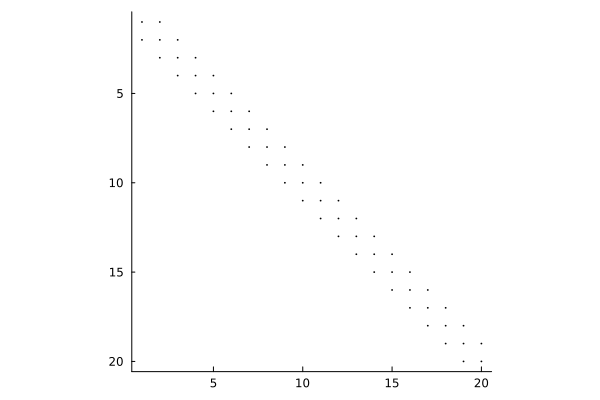
Sparse matrix#

Sparse Hessian matrix of the Hessian matrix of the Rosenbrock function w.r.t. to vector components.

hes_sp = Symbolics.hessian_sparsity(rosenbrock, xs)

20×20 SparseArrays.SparseMatrixCSC{Bool, Int64} with 58 stored entries:
⎡⠻⣦⡀⠀⠀⠀⠀⠀⠀⠀⎤
⎢⠀⠈⠻⣦⡀⠀⠀⠀⠀⠀⎥
⎢⠀⠀⠀⠈⠻⣦⡀⠀⠀⠀⎥
⎢⠀⠀⠀⠀⠀⠈⠻⣦⡀⠀⎥
⎣⠀⠀⠀⠀⠀⠀⠀⠈⠻⣦⎦

Visualize the sparse matrix with Plots.spy()

using Plots
spy(hes_sp)

../_images/f52d4518e711d429b941280d703d4f75ada1866b2b0d90badbeb7edf6d99b41f.png

Generate functions symbolically#

https://docs.sciml.ai/Symbolics/stable/manual/build_function/

build_function(ex, args...) generates out-of-place (oop) and in-place (ip) function expressions in a tuple pair.
build_function(ex, args..., parallel=Symbolics.MultithreadedForm()) generates a parallel, multithreaded algorithm.
build_function(ex, args..., target=Symbolics.CTarget()) generates a C function from Julia.

For example, we want to build a Julia function from grad.

fexprs = build_function(grad, xs);

Get the Out-of-place f(input) version

foop = eval(fexprs[1])

#3 (generic function with 1 method)

Get the In-place f!(out, in) version

fip = eval(fexprs[2])

#5 (generic function with 1 method)

inxs = rand(N)
out = similar(inxs)
fip(out, inxs)  ## The inplace version returns nothing. The results are stored in out parameter.

20-element Vector{Float64}:
  157.35533084647494
 -103.91378308259812
    6.712704680676648
    6.932609921943186
   23.800540958336178
   26.751210335685794
  -35.595656272595036
   39.0861293208317
   37.559507028869405
  -35.521117547121975
  -39.48617284857703
  111.2804937355183
 -108.21815923481964
   -1.2889368056793131
  115.31848217997978
  -52.68545296315378
   95.14630577628606
  -98.28547635929587
   -6.5928820891437
   88.64121296291844

foop(inxs)
isapprox(foop(inxs), out)

true

To save the generated function for later use:

write("function.jl", string(fexprs[2]))

Load it back

g = include("function.jl")

Here, ForwardDiff.jl checks if our gradient generated from Symbolics.jl is correct.

using ForwardDiff: gradient
gradient(rosenbrock, inxs) ≈ out

true

Sparse Hessian matrix, only non-zero expressions are calculated.

hexprs = build_function(hes_sp, xs)
hoop = eval(hexprs[1])
hip = eval(hexprs[2])
hoop(rand(N))

20×20 SparseArrays.SparseMatrixCSC{Bool, Int64} with 58 stored entries:
⎡⠻⣦⡀⠀⠀⠀⠀⠀⠀⠀⎤
⎢⠀⠈⠻⣦⡀⠀⠀⠀⠀⠀⎥
⎢⠀⠀⠀⠈⠻⣦⡀⠀⠀⠀⎥
⎢⠀⠀⠀⠀⠀⠈⠻⣦⡀⠀⎥
⎣⠀⠀⠀⠀⠀⠀⠀⠈⠻⣦⎦

Solve equations symbolically#

https://docs.sciml.ai/Symbolics/stable/manual/solver/

Use symbolic_solve(expr, x) to get analytic solutions.

For single variable solving, the Nemo.jl package is needed; for multiple variable solving, the Groebner.jl package is needed.

This example solves the steady-state rate of a enzyme-catalyzed reaction of fumarate hydratase: https://bmcbioinformatics.biomedcentral.com/articles/10.1186/1471-2105-10-238. At steady-state, the rate of change of each state shoul be zero.

using Symbolics
using Groebner

@variables k1 k2 k3 k4 k5 k6 km1 km2 km3 km4 km5 km6 E1 E2 E3 E4 E5

eqs = let
    v12 = km6 * E1 - k6 * E2
    v13 = k1 * E1 - km1 * E3
    v15 = k3 * E1 - km3 * E5
    v24 = km5 * E2 - k5 * E4
    v34 = k2 * E3 - km2 * E4
    v45 = km4 * E4 - k4 * E5

    dE1 = -v12 - v13 - v15
    dE2 = v12 - v24
    dE3 = v13 - v34
    dE4 = v24 + v34 - v45
    dE5 = v15 + v45

    # Make sure the rates are conserved
    @assert isequal(dE1 + dE2 + dE3 + dE4 + dE5, 0)
    # The following terms should be all zeroes.
    [dE1, dE2, dE3, dE4, E1 + E2 + E3 + E4 + E5 - 1 ]
end

@time sol = Symbolics.symbolic_solve(eqs, [E1, E2, E3, E4, E5])[1]

 37.420144 seconds (123.44 M allocations: 5.187 GiB, 2.41% gc time, 83.18% compilation time: 14% of which was recompilation)

Dict{Symbolics.Num, Any} with 5 entries:
  E4 => (k1*k2*k4*k6 + k1*k2*k4*km5 + k1*k2*k6*km3 + k1*k2*km3*km5 + k2*k3*k4*k…
  E5 => (k1*k2*k6*km4 + k1*k2*km4*km5 + k2*k3*k5*k6 + k2*k3*k6*km4 + k2*k3*km4*…
  E2 => (k1*k2*k4*k5 + k1*k2*k5*km3 + k2*k3*k4*k5 + k2*k4*k5*km6 + k2*k5*km3*km…
  E1 => (k2*k4*k5*k6 + k2*k5*k6*km3 + k2*k6*km3*km4 + k2*km3*km4*km5 + k4*k5*k6…
  E3 => (k1*k4*k5*k6 + k1*k4*k6*km2 + k1*k4*km2*km5 + k1*k5*k6*km3 + k1*k6*km2*…

The weight of the first enzyme state is

numerator(sol[E1])

\[ \begin{equation} \mathtt{k2} \mathtt{k4} \mathtt{k5} \mathtt{k6} + \mathtt{k2} \mathtt{k5} \mathtt{k6} \mathtt{km3} + \mathtt{k2} \mathtt{k6} \mathtt{km3} \mathtt{km4} + \mathtt{k2} \mathtt{km3} \mathtt{km4} \mathtt{km5} + \mathtt{k4} \mathtt{k5} \mathtt{k6} \mathtt{km1} + \mathtt{k4} \mathtt{k6} \mathtt{km1} \mathtt{km2} + \mathtt{k4} \mathtt{km1} \mathtt{km2} \mathtt{km5} + \mathtt{k5} \mathtt{k6} \mathtt{km1} \mathtt{km3} + \mathtt{k6} \mathtt{km1} \mathtt{km2} \mathtt{km3} + \mathtt{k6} \mathtt{km1} \mathtt{km3} \mathtt{km4} + \mathtt{km1} \mathtt{km2} \mathtt{km3} \mathtt{km5} + \mathtt{km1} \mathtt{km3} \mathtt{km4} \mathtt{km5} \end{equation} \]

This notebook was generated using Literate.jl.