Tips

Differentiable smooth functions

Smooth and differentiable functions are more friendly for automatic differentiation (AD) and differential equation solvers.

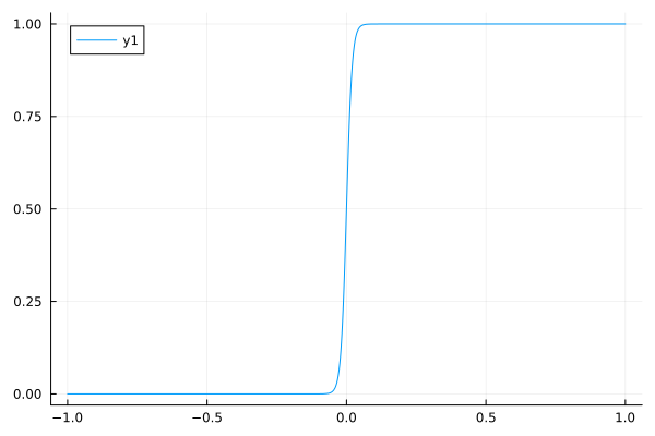
Smooth Heaviside step function

A Heaviside step function (0 when x < a, 1 when x > a) could be approximated with a steep logistic function.

using Plots

The function output switches from zero to one around x=0.

function smoothheaviside(x, k=100)
    1 / (1 + exp(-k * x))
end

plot(smoothheaviside, -1, 1)

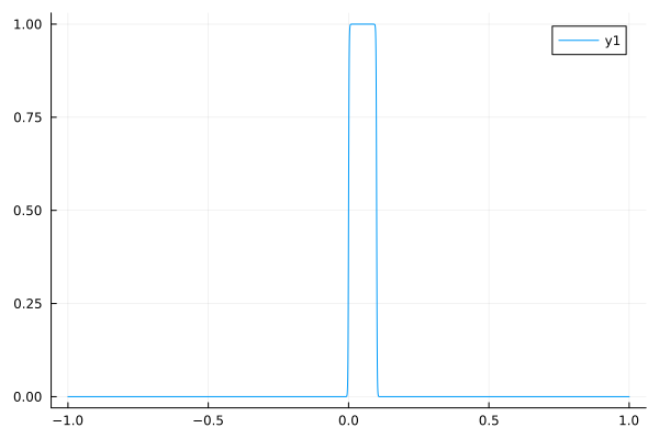
Smooth single pulse

A single pulse could be approximated with a product of two logistic functions.

function singlepulse(x, t0=0, t1=0.1, k=1000)
    smoothheaviside(x - t0, k) * smoothheaviside(t1 - x, k)
end

plot(singlepulse, -1, 1)

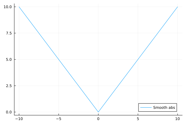
Smooth absolute value

Inspired by: https://discourse.julialang.org/t/smooth-approximation-to-max-0-x/109383/13

# Approximate abs(x)
function smooth_abs(x; c=(1//2)^10)
    sqrt(x^2 + c^2) - c
end

plot(smooth_abs, -10, 10, label="Smooth abs")

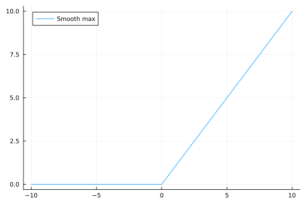
Smooth max function

Approximate max(0, x)

function smooth_max(x; c=(1//2)^10)
    0.5 * (x + smooth_abs(x;c))
end

plot(smooth_max, -10, 10, label="Smooth max")

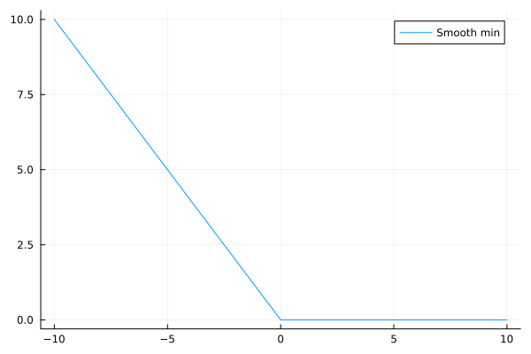
Smooth minimal function

Approximate min(0, x)

function smooth_min(x; c=(1//2)^10)
    0.5 * (smooth_abs(x;c) - x)
end

plot(smooth_min, -10, 10, label="Smooth min")

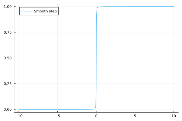
(Another) smooth step function

function smooth_step(x; c=(1//2)^10)
    0.5 * (x / (sqrt(x^2 + c)) + 1)
end

plot(smooth_step, -10, 10, label="Smooth step")

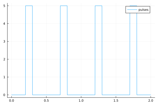
Periodic pulses

From: https://www.noamross.net/2015/11/12/a-smooth-differentiable-pulse-function/

function smoothpulses(t, tstart, tend, period=1, amplitude=period / (tend - tstart), steepness=1000)
    @assert tstart < tend < period
    xi = 3 / 4 - (tend - tstart) / (2 * period)
    p = inv(1 + exp(steepness * (sinpi(2 * ((t - tstart) / period + xi)) - sinpi(2 * xi))))
    return amplitude * p
end

plot(t->smoothpulses(t, 0.2, 0.3, 0.5), 0.0, 2.0, lab="pulses")

Avoid DomainErrors

Some functions such as sqrt(x), log(x), and pow(x), throw DomainError exceptions with negative x, interrupting differential equation solvers. One can use the respective functions in JuliaMath/NaNMath.jl, returning NaN instead of throwing a DomainError. Then, the differential equation solvers will reject the solution and retry with a smaller time step.

import NaNMath as nm
nm.sqrt(-1.0) ## returns NaN

# ODE function from an MTK ODE system

NaN

f = ODEFunction(sys) could be useful in visualizing vector fields.

using ModelingToolkit
using OrdinaryDiffEq
using Plots

@independent_variables t
@variables x(t) RHS(t)
@parameters τ
D = Differential(t)

Differential(t)

Equations in MTK use the tilde character (~) as equality. Every MTK system requires a name. The @named macro simply ensures that the symbolic name matches the name in the REPL.

eqs = [
    RHS  ~ (1 - x)/τ,
    D(x) ~ RHS
]

@mtkbuild fol_separate = ODESystem(eqs, t)
f = ODEFunction(fol_separate)

(::SciMLBase.ODEFunction{true, SciMLBase.AutoSpecialize, ModelingToolkit.GeneratedFunctionWrapper{(2, 3, true), RuntimeGeneratedFunctions.RuntimeGeneratedFunction{(:__mtk_arg_1, :___mtkparameters___, :t), ModelingToolkit.var"#_RGF_ModTag", ModelingToolkit.var"#_RGF_ModTag", (0x87998280, 0x468561ce, 0x00d5cbc8, 0x1505867c, 0x1afd5a12), Nothing}, RuntimeGeneratedFunctions.RuntimeGeneratedFunction{(:ˍ₋out, :__mtk_arg_1, :___mtkparameters___, :t), ModelingToolkit.var"#_RGF_ModTag", ModelingToolkit.var"#_RGF_ModTag", (0x29f228b0, 0xf411e595, 0xafb12892, 0x0abf7abb, 0xef8266d7), Nothing}}, LinearAlgebra.UniformScaling{Bool}, Nothing, Nothing, Nothing, Nothing, Nothing, Nothing, Nothing, Nothing, Nothing, Nothing, Nothing, ModelingToolkit.ObservedFunctionCache{ModelingToolkit.ODESystem}, Nothing, ModelingToolkit.ODESystem, Nothing, Nothing}) (generic function with 1 method)

f(u, p, t) returns the value of derivatives

f([0.0], [1.0], 0.0)

1-element Vector{Float64}:
 1.0

If you already have the ODEproblem, the function is prob.f.

prob = ODEProblem(fol_separate, [x => 0.0], (0.0, 1.0), [τ => 1.0])
f = prob.f
f([0.0], [1.0], 0.0)

1-element Vector{Float64}:
 1.0

---

This notebook was generated using Literate.jl.