Callbacks and Events

Docs:

• https://docs.sciml.ai/DiffEqDocs/stable/features/callback_functions/

• https://tutorials.sciml.ai/html/introduction/04-callbacks_and_events.html

Types

• ContinuousCallback: applied when a given continuous condition function hits zero. SciML solvers are able to interpolate the integration step to meet the condition.

• DiscreteCallback: applied when its condition function is true.

• CallbackSet(cb1, cb2, ...): Multiple callbacks can be chained together to form a CallbackSet.

• VectorContinuousCallback: an array of ContinuousCallbacks.

How to

After you define a callback, send it to the solve() function:

sol = solve(prob, alg, callback=cb)

DiscreteCallback : Interventions at Preset Times

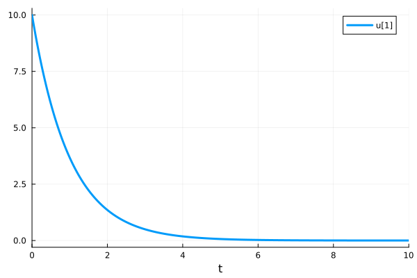
The drug concentration in the blood follows exponential decay.

using OrdinaryDiffEq
using DiffEqCallbacks
using Plots

Exponential decay model

function dosing!(du, u, p, t)
    du[1] = -u[1]
end

u0 = [10.0]
tspan = (0.0, 10.0)
prob = ODEProblem(dosing!, u0, tspan)
sol = solve(prob, Tsit5())

plot(sol, lw=3)

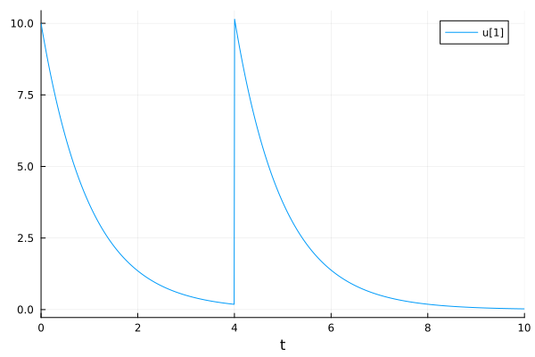
Add a dose of 10 at t = 4. You may need to force the solver to stop at t==4 by using tstops=[4.0] to properly apply the callback.

condition(u, t, integrator) = t == 4
affect!(integrator) = integrator.u[1] += 10
cb = DiscreteCallback(condition, affect!)

sol = solve(prob, Tsit5(), callback=cb, tstops=[4.0])
plot(sol)

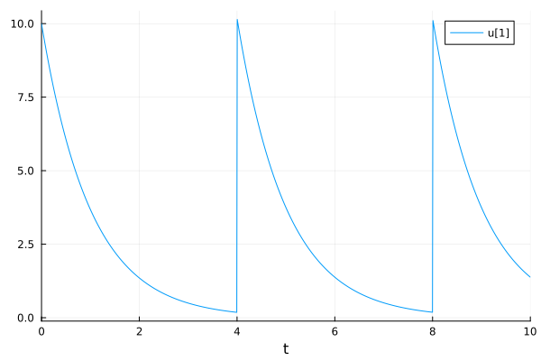
Applying multiple doses.

dosetimes = [4.0, 8.0]
condition(u, t, integrator) = t ∈ dosetimes
affect!(integrator) = integrator.u[1] += 10
cb = DiscreteCallback(condition, affect!)

sol = solve(prob, Tsit5(), callback=cb, tstops=dosetimes)
plot(sol)

Conditional dosing. Note that a dose was not given at t=6 because the concentration is not more than 1.

dosetimes = [4.0, 6.0, 8.0]
condition(u, t, integrator) = t ∈ dosetimes && (u[1] < 1.0)
affect!(integrator) = integrator.u[1] += 10integrator.t
cb = DiscreteCallback(condition, affect!)

sol = solve(prob, Tsit5(), callback=cb, tstops=dosetimes)
plot(sol)

PresetTimeCallback

PresetTimeCallback(tstops, affect!) takes an array of times and an affect! function to apply. The solver will stop at tstops to ensure callbacks are applied.

dosetimes = [4.0, 8.0]
affect!(integrator) = integrator.u[1] += 10
cb = PresetTimeCallback(dosetimes, affect!)
sol = solve(prob, Tsit5(), callback=cb)
plot(sol)

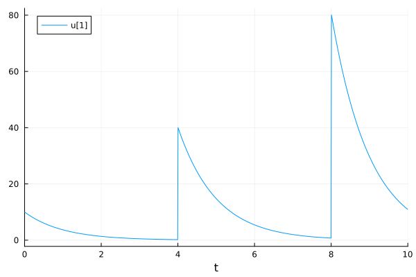
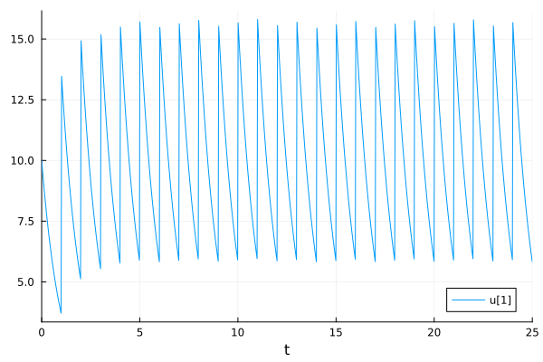
Periodic callback

PeriodicCallback is a special case of DiscreteCallback, used when a function should be called periodically in terms of integration time (as opposed to wall time).

prob = ODEProblem(dosing!, u0, (0.0, 25.0))

affect!(integrator) = integrator.u[1] += 10
cb = PeriodicCallback(affect!, 1.0)

sol = solve(prob, Tsit5(), callback=cb)
plot(sol)

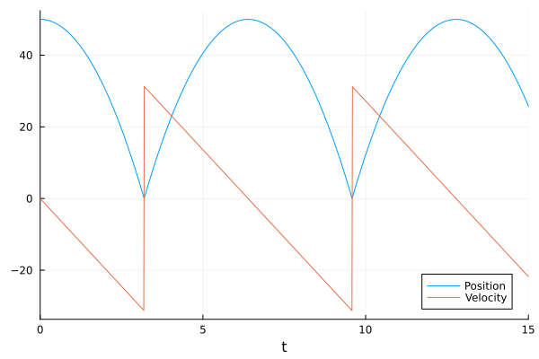
Continuous Callback

bouncing Ball example

using OrdinaryDiffEq
using DiffEqCallbacks
using Plots

function ball!(du, u, p, t)
    du[1] = u[2]
    du[2] = -p
end

# When the ball touches the ground
# Telling when event_f(u,t) == 0
function condition(u, t, integrator)
    u[1]
end

function affect!(integrator)
    integrator.u[2] = -integrator.u[2]
end

cb = ContinuousCallback(condition, affect!)

u0 = [50.0, 0.0]
tspan = (0.0, 15.0)
p = 9.8

prob = ODEProblem(ball!, u0, tspan, p)
sol = solve(prob, Tsit5(), callback=cb)
plot(sol, label=["Position" "Velocity"])

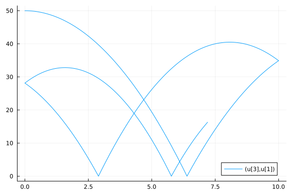
Vector Continuous Callback

You can group multiple callbacks together into a vector. In this example, we will simulate bouncing ball with multiple walls.

using OrdinaryDiffEq
using DiffEqCallbacks
using Plots

function ball_2d!(du, u, p, t)
    du[1] = u[2]  ## x_pos
    du[2] = -p    ## x_vel
    du[3] = u[4]  ## y_pos
    du[4] = 0.0   ## y_vel
end

ball_2d! (generic function with 1 method)

Vector conditions

function condition(out, u, t, integrator) ## Event when event_f(u,t) == 0
    out[1] = u[1]
    out[2] = (u[3] - 10.0)u[3]
end

condition (generic function with 2 methods)

Vector affects

function affect!(integrator, idx)
    if idx == 1
        integrator.u[2] = -0.9integrator.u[2]
    elseif idx == 2
        integrator.u[4] = -0.9integrator.u[4]
    end
end

cb = VectorContinuousCallback(condition, affect!, 2)
u0 = [50.0, 0.0, 0.0, 2.0]
tspan = (0.0, 15.0)
p = 9.8
prob = ODEProblem(ball_2d!, u0, tspan, p)
sol = solve(prob, Tsit5(), callback=cb, dt=1e-3, adaptive=false)
plot(sol, idxs=(3, 1))

Other Callbacks

https://diffeq.sciml.ai/stable/features/callback_library/

• ManifoldProjection(g): keep g(u) = 0 for energy conservation.

• AutoAbstol(): automatically adapt the absolute tolerance.

• PositiveDomain(): enforce non-negative solution. The system should also be defined outside the positive domain. There is also a more general version GeneralDomain().

• StepsizeLimiter((u,p,t) -> maxtimestep): restrict maximal allowed time step.

• FunctionCallingCallback((u, t, int) -> func_content; funcat=[t1, t2, ...]): call a function at the time points (t1, t2, …) of interest.

• SavingCallback((u, t, int) -> data_to_be_saved, dataprototype): call a function and saves the result.

• IterativeCallback(time_choice(int) -> t2, user_affect!): apply an effect at the time of the next callback.

---

This notebook was generated using Literate.jl.