Bayesian inference for PINNs

https://docs.sciml.ai/NeuralPDE/stable/tutorials/Lotka_Volterra_BPINNs/

using NeuralPDE
using AdvancedHMC
using MCMCChains
using LogDensityProblems
using Lux
using Plots
using OrdinaryDiffEq
using Distributions
using Random

rng = Random.default_rng()
Random.seed!(rng, 42)

Random.TaskLocalRNG()

NNODE only supports out-of-place functions f(u, p ,t)

function lotka_volterra(u, p, t)
    # Model parameters.
    α, β, γ, δ = p
    # Current state.
    x, y = u

    # Evaluate differential equations.
    dx = (α - β * y) * x ## prey
    dy = (δ * x - γ) * y ## predator

    return [dx, dy]
end

lotka_volterra (generic function with 1 method)

Reference solution for the Lotka-Volterra system

u0 = [1.0, 1.0]
p = [1.5, 1.0, 3.0, 1.0]
tspan = (0.0, 4.0)
prob = ODEProblem(lotka_volterra, u0, tspan, p)
dt = 0.01
solution = solve(prob, Tsit5(); saveat = dt)

retcode: Success
Interpolation: 1st order linear
t: 401-element Vector{Float64}:
 0.0
 0.01
 0.02
 0.03
 0.04
 0.05
 0.06
 0.07
 0.08
 0.09
 ⋮
 3.92
 3.93
 3.94
 3.95
 3.96
 3.97
 3.98
 3.99
 4.0
u: 401-element Vector{Vector{Float64}}:
 [1.0, 1.0]
 [1.0051122697054304, 0.9802235489841001]
 [1.0104482482084793, 0.9608884029133249]
 [1.0160067852516195, 0.9419859539931972]
 [1.0217868581271055, 0.9235077034160883]
 [1.0277875716769742, 0.9054452613612181]
 [1.0340081582930438, 0.887790346994655]
 [1.040447977916915, 0.870534788469315]
 [1.0471065141055134, 0.8536705240234226]
 [1.0539833005834183, 0.837189627503347]
 ⋮
 [1.7188602790655703, 0.35603128520071003]
 [1.7386754231380195, 0.35153232204585927]
 [1.7587969344457686, 0.3471593575148184]
 [1.779227949981121, 0.34291022060855736]
 [1.7999716537968578, 0.3387828301940905]
 [1.821031277006269, 0.3347751950044705]
 [1.8424100977831226, 0.3308854136387941]
 [1.8641114413617017, 0.3271116745621956]
 [1.886138680036769, 0.32345225610585315]

Dataset creation for parameter estimation (plus 30% noise)

time = solution.t
u = hcat(solution.u...)
x = u[1, :] + (u[1, :]) .* (0.3 .* randn(length(u[1, :])))
y = u[2, :] + (u[2, :]) .* (0.3 .* randn(length(u[2, :])))
dataset = [x, y, time]

# Plotting the data which will be used
plot(time, x, label = "noisy x")
plot!(time, y, label = "noisy y")
plot!(solution, labels = ["x" "y"])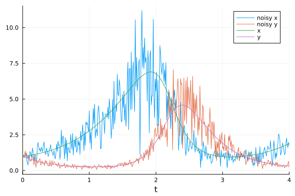

Define a PINN neural network. The input is time, and the output is the state of the system (x and y).

chain = Chain(Dense(1, 6, tanh), Dense(6, 6, tanh), Dense(6, 2))

Chain(
    layer_1 = Dense(1 => 6, tanh),                # 12 parameters
    layer_2 = Dense(6 => 6, tanh),                # 42 parameters
    layer_3 = Dense(6 => 2),                      # 14 parameters
)         # Total: 68 parameters,
          #        plus 0 states.

Use BNNODE for Bayesian inference. The parameters of the model are estimated with the dataset, and the uncertainty of the estimation is quantified with the posterior distribution.

alg = BNNODE(chain;
    dataset = dataset,
    draw_samples = 1000,
    l2std = [0.1, 0.1],
    phystd = [0.1, 0.1],
    priorsNNw = (0.0, 3.0),
    param = [
        Normal(1, 2),
        Normal(2, 2),
        Normal(2, 2),
        Normal(0, 2)],
    progress = false
)

NeuralPDE.BNNODE{Lux.Chain{@NamedTuple{layer_1::Lux.Dense{typeof(tanh), Int64, Int64, Nothing, Nothing, Static.True}, layer_2::Lux.Dense{typeof(tanh), Int64, Int64, Nothing, Nothing, Static.True}, layer_3::Lux.Dense{typeof(identity), Int64, Int64, Nothing, Nothing, Static.True}}, Nothing}, UnionAll, Nothing, Vector{Distributions.Normal{Float64}}, NeuralPDEBPINNExt.var"#27#28", Vector{Vector{Float64}}, @NamedTuple{n_leapfrog::Int64}, Nothing, @NamedTuple{Adaptor::UnionAll, Metric::UnionAll, targetacceptancerate::Float64}, @NamedTuple{Integrator::UnionAll}}(Lux.Chain{@NamedTuple{layer_1::Lux.Dense{typeof(tanh), Int64, Int64, Nothing, Nothing, Static.True}, layer_2::Lux.Dense{typeof(tanh), Int64, Int64, Nothing, Nothing, Static.True}, layer_3::Lux.Dense{typeof(identity), Int64, Int64, Nothing, Nothing, Static.True}}, Nothing}((layer_1 = Dense(1 => 6, tanh), layer_2 = Dense(6 => 6, tanh), layer_3 = Dense(6 => 2)), nothing), AdvancedHMC.HMC, nothing, 1000, (0.0, 3.0), Distributions.Normal{Float64}[Distributions.Normal{Float64}(μ=1.0, σ=2.0), Distributions.Normal{Float64}(μ=2.0, σ=2.0), Distributions.Normal{Float64}(μ=2.0, σ=2.0), Distributions.Normal{Float64}(μ=0.0, σ=2.0)], [0.1, 0.1], [0.1, 0.1], NeuralPDEBPINNExt.var"#27#28"(), [[0.8909927555644668, 1.081019518939972, 0.9149645351061549, 0.921136419750178, 1.2720143155095367, 1.1747833061967605, 0.7673719750261206, 0.5818325951979773, 0.382926381702283, 1.0678268427790336  …  1.7257325742047445, 1.4318373311301964, 1.1138322647569558, 1.1810578269152001, 1.852781536639801, 2.2714964425464856, 1.8427223212379569, 1.6125087985762456, 1.978075036427335, 1.7692283839290162], [0.7435691922373409, 1.0416345182191378, 1.0872852706814091, 1.0755362585523962, 1.372372556710778, 0.9816260007024543, 1.2335800497364675, 0.865342928800918, 0.988618315274289, 0.9012588979308397  …  0.38626397872695484, 0.3727453510366658, 0.1868940104993419, 0.2998216413303031, 0.29188996818212654, 0.27876359043859084, 0.39633723208305116, 0.4533106790699501, 0.6366272958591013, 0.19871401559731644], [0.0, 0.01, 0.02, 0.03, 0.04, 0.05, 0.06, 0.07, 0.08, 0.09  …  3.91, 3.92, 3.93, 3.94, 3.95, 3.96, 3.97, 3.98, 3.99, 4.0]], 0.05, (n_leapfrog = 30,), 1, nothing, (Adaptor = AdvancedHMC.Adaptation.StanHMCAdaptor, Metric = AdvancedHMC.DiagEuclideanMetric, targetacceptancerate = 0.8), (Integrator = AdvancedHMC.Leapfrog,), 333, false, false, false, false)

Solve the problem

@time sol_pestim = solve(prob, alg; saveat = dt)
sol_pestim.estimated_de_params

358.240235 seconds (291.43 M allocations: 1.101 TiB, 27.37% gc time, 3.73% compilation time)

4-element Vector{MonteCarloMeasurements.Particles{Float64, 334}}:
 0.439 ± 0.11
 0.14 ± 0.031
 0.313 ± 0.15
 0.231 ± 0.059

Visualize the fit

plot(time, sol_pestim.ensemblesol[1], label = "estimated x")
plot!(time, sol_pestim.ensemblesol[2], label = "estimated y")
plot!(solution, labels = ["true x" "true y"])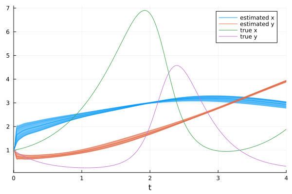

This notebook was generated using Literate.jl.