Multiple Shooting - Julia UDE

Docs: https://docs.sciml.ai/DiffEqFlux/dev/examples/multiple_shooting/

In Multiple Shooting, the training data is split into overlapping intervals. The solver (OptimizationPolyalgorithms.PolyOpt()) is trained on individual intervals. The results are stiched together.

This simple method assumes no noise in the data. A more robust version can be found at JuliaSimModelOptimizer.jl, which is a proprietary software.

using ComponentArrays
using DiffEqFlux
using DiffEqFlux: group_ranges
using Lux
using Optimization
using OptimizationPolyalgorithms
using OrdinaryDiffEq
using Plots
using Random
rng = Random.Xoshiro(0)

Random.Xoshiro(0xdb2fa90498613fdf, 0x48d73dc42d195740, 0x8c49bc52dc8a77ea, 0x1911b814c02405e8, 0x22a21880af5dc689)

Define initial conditions and time steps

datasize = 51
u0 = Float32[2.0, 0.0]
tspan = (0.0f0, 5.0f0)
tsteps = range(tspan[begin], tspan[end], length = datasize)

0.0f0:0.1f0:5.0f0

Generate data from the true function: $x^3 * A$

function trueODEfunc!(du, u, p, t; true_A = Float32[-0.1 2.0; -2.0 -0.1])
    du .= ((u.^3)'true_A)'
end

prob_trueode = ODEProblem(trueODEfunc!, u0, tspan)
ode_data = Array(solve(prob_trueode, Tsit5(), saveat = tsteps))

┌ Warning: Verbosity toggle: dt_epsilon 
│  Initial timestep too small (near machine epsilon), using default: dt = 1.0e-6
└ @ OrdinaryDiffEqCore ~/.julia/packages/OrdinaryDiffEqCore/rnOL4/src/initdt.jl:196

2×51 Matrix{Float32}:
 2.0  1.76453  0.666819  -0.580549  …  0.0619097  -0.107015  -0.271154
 0.0  1.4286   1.86579    1.80632      0.949526    0.941073   0.931262

Define the Neural Network using Lux.jl

nn = Lux.Chain(
    x -> x.^3,
    Lux.Dense(2, 16, tanh),
    Lux.Dense(16, 2)
)
p_init, st = Lux.setup(rng, nn)
ps = ComponentArray(p_init)
pd, pax = getdata(ps), getaxes(ps)

(Float32[-1.8019577, -0.18273845, 1.677652, 0.19449931, 0.7557112, 1.1159611, -1.581186, 1.7986798, -0.36156967, -1.9202054  …  0.35582402, -0.29064924, 0.32653868, 0.36876014, -0.35387143, 0.12959939, 0.25605455, -0.20957911, 0.10817152, -0.20544955], (Axis(layer_1 = ViewAxis(1:0, Shaped1DAxis((0,))), layer_2 = ViewAxis(1:48, Axis(weight = ViewAxis(1:32, ShapedAxis((16, 2))), bias = ViewAxis(33:48, Shaped1DAxis((16,))))), layer_3 = ViewAxis(49:82, Axis(weight = ViewAxis(1:32, ShapedAxis((2, 16))), bias = ViewAxis(33:34, Shaped1DAxis((2,)))))),))

Define the NeuralODE problem

neuralode = NeuralODE(nn, tspan, Tsit5(), saveat = tsteps)
prob_node = ODEProblem((u,p,t)->nn(u,p,st)[1], u0, tspan, ComponentArray(p_init))

ODEProblem with uType Vector{Float32} and tType Float32. In-place: false
Non-trivial mass matrix: false
timespan: (0.0f0, 5.0f0)
u0: 2-element Vector{Float32}:
 2.0
 0.0

Parameters for Multiple Shooting

group_size = 3
continuity_term = 200  ## Penalty for discontinuity

function loss_function(data, pred)
    return sum(abs2, data .- pred)
end

l1, preds = multiple_shoot(ps, ode_data, tsteps, prob_node, loss_function, Tsit5(), group_size; continuity_term)

function loss_multiple_shooting(theta)
    ps = ComponentArray(theta, pax)
    loss, currpred = multiple_shoot(ps, ode_data, tsteps, prob_node, loss_function,
        Tsit5(), group_size; continuity_term)
    return loss
end

loss_multiple_shooting (generic function with 1 method)

Animate training process in the callback function

function plot_multiple_shoot(plt, preds, group_size)
	ranges = group_ranges(datasize, group_size)
	for (i, rg) in enumerate(ranges)
		plot!(plt, tsteps[rg], preds[i][1,:], markershape=:circle, label="Group $(i)")
	end
end

anim = Animation()
lossrecord=Float64[]
callback = function (state, l; doplot = true, prob_node = prob_node)
    if doplot
        l1, preds = multiple_shoot(
            ComponentArray(state.u, pax), ode_data, tsteps, prob_node, loss_function,
            Tsit5(), group_size; continuity_term)
        plt = scatter(tsteps, ode_data[1,:], label = "Data")
        plot_multiple_shoot(plt, preds, group_size)
        frame(anim)
        push!(lossrecord, l)
    end
    return false
end

#10 (generic function with 1 method)

Solve the problem using OptimizationPolyalgorithms.PolyOpt().

adtype = Optimization.AutoZygote()
optf = Optimization.OptimizationFunction((x,p) -> loss_multiple_shooting(x), adtype)
optprob = Optimization.OptimizationProblem(optf, pd)
@time res_ms = Optimization.solve(optprob, PolyOpt(), callback = callback, maxiters = 300)

println("Loss is ", loss_multiple_shooting(res_ms.u)[1])

134.680668 seconds (471.87 M allocations: 29.129 GiB, 4.58% gc time, 63.45% compilation time: 4% of which was recompilation)
Loss is 11.947134

Loss over epochs

plot(lossrecord, yscale=:log10, label="Loss", xlabel="Iterations", ylabel="Loss (log10)", title="Loss over iterations")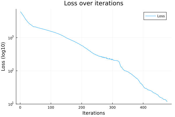

Visualize the fitting processes

mp4(anim, fps=15)

[ Info: Saved animation to /tmp/jl_DcP45k3sfi.mp4

This notebook was generated using Literate.jl.