1D PDE: SIS diffusion model#
where \(x \in (0, 1)\)
Solve the steady-state problem \(\frac{\partial S}{\partial t} = \frac{\partial I}{\partial t} = 0\)
The boundary condition: \(\frac{\partial S}{\partial x} = \frac{\partial I}{\partial x} = 0\) for x = 0, 1
The conservative relationship: \(\int^{1}_{0} (S(x) + I(x) ) dx = 1\)
Notations:
\(x\) : location
\(t\) : time
\(S(x, t)\) : the density of susceptible populations
\(I(x, t)\) : the density of infected populations
\(d_S\) / \(d_I\) : the diffusion coefficients for susceptible and infected individuals
\(\beta(x)\) : transmission rates
\(\gamma(x)\) : recovery rates
using OrdinaryDiffEq
using ModelingToolkit
using MethodOfLines
using DomainSets
using Plots
Setup parameters, variables, and differential operators
@parameters t x
@parameters dS dI brn ϵ
@variables S(..) I(..)
Dt = Differential(t)
Dx = Differential(x)
Dxx = Differential(x)^2
Differential(x) ∘ Differential(x)
Helper functions
γ(x) = x + 1
ratio(x, brn, ϵ) = brn + ϵ * sinpi(2x)
ratio (generic function with 1 method)
1D PDE for disease spreading
eqs = [
    Dt(S(t, x)) ~ dS * Dxx(S(t, x)) - ratio(x, brn, ϵ) * γ(x) * S(t, x) * I(t, x) / (S(t, x) + I(t, x)) + γ(x) * I(t, x),
    Dt(I(t, x)) ~ dI * Dxx(I(t, x)) + ratio(x, brn, ϵ) * γ(x) * S(t, x) * I(t, x) / (S(t, x) + I(t, x)) - γ(x) * I(t, x)
]
Boundary conditions
bcs = [
    S(0, x) ~ 0.9 + 0.1 * sinpi(2x),
    I(0, x) ~ 0.1 + 0.1 * cospi(2x),
    Dx(S(t, 0)) ~ 0.0,
    Dx(S(t, 1)) ~ 0.0,
    Dx(I(t, 0)) ~ 0.0,
    Dx(I(t, 1)) ~ 0.0
]
Space and time domains
domains = [
    t ∈ Interval(0.0, 10.0),
    x ∈ Interval(0.0, 1.0)
]
2-element Vector{Symbolics.VarDomainPairing}:
 Symbolics.VarDomainPairing(t, 0.0 .. 10.0)
 Symbolics.VarDomainPairing(x, 0.0 .. 1.0)
Build the PDE system
@named pdesys = PDESystem(eqs, bcs, domains,
    [t, x], ## Independent variables
    [S(t, x), I(t, x)],  ## Dependent variables
    [dS, dI, brn, ϵ],    ## parameters
    defaults = Dict(dS => 0.5, dI => 0.1, brn => 3, ϵ => 0.1)
)
Finite difference method (FDM) converts the PDE system into an ODE problem
dx = 0.01
order = 2
discretization = MOLFiniteDifference([x => dx], t, approx_order=order)
prob = discretize(pdesys, discretization)
ODEProblem with uType Vector{Float64} and tType Float64. In-place: true
Non-trivial mass matrix: false
timespan: (0.0, 10.0)
u0: 198-element Vector{Float64}:
 0.19980267284282716
 0.1992114701314478
 0.19822872507286887
 0.1968583161128631
 0.19510565162951538
 0.19297764858882513
 0.190482705246602
 0.18763066800438638
 0.18443279255020154
 0.18090169943749476
 ⋮
 0.9535826794978997
 0.9481753674101716
 0.9425779291565073
 0.9368124552684678
 0.9309016994374948
 0.9248689887164855
 0.9187381314585725
 0.9125333233564304
 0.9062790519529313
Solving time-dependent SIS epidemic model#
KenCarp4 is good at solving semilinear problems (like reaction-diffusion problems).
sol = solve(prob, KenCarp4(), saveat=0.2)
retcode: Success
Interpolation: Dict{Symbolics.Num, Interpolations.GriddedInterpolation{Float64, 2, Matrix{Float64}, Interpolations.Gridded{Interpolations.Linear{Interpolations.Throw{Interpolations.OnGrid}}}, Tuple{Vector{Float64}, Vector{Float64}}}}
t: 51-element Vector{Float64}:
  0.0
  0.2
  0.4
  0.6
  0.8
  1.0
  1.2
  1.4
  1.6
  1.8
  ⋮
  8.4
  8.6
  8.8
  9.0
  9.2
  9.4
  9.6
  9.8
 10.0ivs: 2-element Vector{SymbolicUtils.BasicSymbolic{Real}}:
 t
 xdomain:([0.0, 0.2, 0.4, 0.6, 0.8, 1.0, 1.2, 1.4, 1.6, 1.8  …  8.2, 8.4, 8.6, 8.8, 9.0, 9.2, 9.4, 9.6, 9.8, 10.0], 0.0:0.01:1.0)
u: Dict{Symbolics.Num, Matrix{Float64}} with 2 entries:
  S(t, x) => [0.904194 0.906279 … 0.893721 0.895806; 0.879603 0.879585 … 0.7899…
  I(t, x) => [0.2 0.199803 … 0.199803 0.2; 0.204066 0.20397 … 0.245398 0.245559…
Grid points
discrete_x = sol[x]
discrete_t = sol[t]
51-element Vector{Float64}:
  0.0
  0.2
  0.4
  0.6
  0.8
  1.0
  1.2
  1.4
  1.6
  1.8
  ⋮
  8.4
  8.6
  8.8
  9.0
  9.2
  9.4
  9.6
  9.8
 10.0
Results (Matrices)
S_solution = sol[S(t, x)]
I_solution = sol[I(t, x)]
51×101 Matrix{Float64}:
 0.2       0.199803  0.199211  0.198229  …  0.199211  0.199803  0.2
 0.204066  0.20397   0.203684  0.203205     0.244914  0.245398  0.245559
 0.239603  0.239568  0.239463  0.239285     0.320347  0.320719  0.320844
 0.300269  0.300279  0.300309  0.300355     0.413565  0.413853  0.413949
 0.37595   0.375987  0.376098  0.376278     0.503721  0.503946  0.504021
 0.451583  0.451629  0.451768  0.451996  …  0.573511  0.573687  0.573745
 0.516804  0.516848  0.516981  0.517198     0.620077  0.620214  0.62026
 0.566319  0.566357  0.566469  0.566653     0.646894  0.647002  0.647038
 0.601149  0.601179  0.601268  0.601415     0.660188  0.660274  0.660303
 0.624958  0.624981  0.625051  0.625165     0.665471  0.665541  0.665564
 ⋮                                       ⋱                      ⋮
 0.676304  0.676307  0.676318  0.676335     0.656519  0.656544  0.656553
 0.676303  0.676307  0.676318  0.676335     0.656519  0.656544  0.656553
 0.676303  0.676307  0.676317  0.676334     0.656519  0.656544  0.656553
 0.676302  0.676306  0.676317  0.676333  …  0.656519  0.656545  0.656553
 0.676301  0.676305  0.676316  0.676333     0.65652   0.656545  0.656554
 0.676301  0.676304  0.676315  0.676332     0.65652   0.656546  0.656554
 0.6763    0.676304  0.676315  0.676331     0.656521  0.656546  0.656554
 0.6763    0.676304  0.676314  0.676331     0.656521  0.656546  0.656554
 0.6763    0.676304  0.676315  0.676331  …  0.656521  0.656546  0.656554
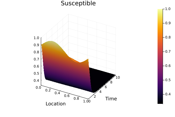
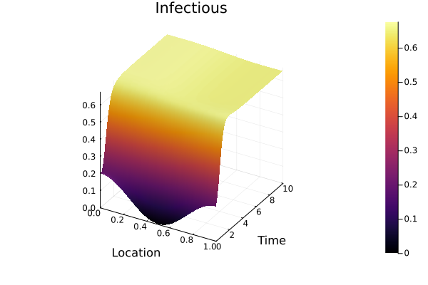
Visualize the solution
surface(discrete_x, discrete_t, S_solution, xlabel="Location", ylabel="Time", title="Susceptible")
surface(discrete_x, discrete_t, I_solution, xlabel="Location", ylabel="Time", title="Infectious")
This notebook was generated using Literate.jl.