Repressilator

Repressilator model consists of a biochemical reaction network with three components in a negative feedback loop.

using Catalyst
using ModelingToolkit
using DifferentialEquations
using Plots

repressilator = @reaction_network begin
    hillr(P₃, α, K, n), ∅ --> m₁
    hillr(P₁, α, K, n), ∅ --> m₂
    hillr(P₂, α, K, n), ∅ --> m₃
    (δ, γ), m₁ ↔ ∅
    (δ, γ), m₂ ↔ ∅
    (δ, γ), m₃ ↔ ∅
    β, m₁ --> m₁ + P₁
    β, m₂ --> m₂ + P₂
    β, m₃ --> m₃ + P₃
    μ, P₁ --> ∅
    μ, P₂ --> ∅
    μ, P₃ --> ∅
end

\[\begin{split} \begin{align*} \varnothing &\xrightarrow{\frac{K^{n} \alpha}{K^{n} + \mathtt{P_3}^{n}}} \mathrm{\mathtt{m_1}} \\ \varnothing &\xrightarrow{\frac{K^{n} \alpha}{\mathtt{P_1}^{n} + K^{n}}} \mathrm{\mathtt{m_2}} \\ \varnothing &\xrightarrow{\frac{K^{n} \alpha}{K^{n} + \mathtt{P_2}^{n}}} \mathrm{\mathtt{m_3}} \\ \mathrm{\mathtt{m_1}} &\xrightleftharpoons[\gamma]{\delta} \varnothing \\ \mathrm{\mathtt{m_2}} &\xrightleftharpoons[\gamma]{\delta} \varnothing \\ \mathrm{\mathtt{m_3}} &\xrightleftharpoons[\gamma]{\delta} \varnothing \\ \mathrm{\mathtt{m_1}} &\xrightarrow{\beta} \mathrm{\mathtt{m_1}} + \mathrm{\mathtt{P_1}} \\ \mathrm{\mathtt{m_2}} &\xrightarrow{\beta} \mathrm{\mathtt{m_2}} + \mathrm{\mathtt{P_2}} \\ \mathrm{\mathtt{m_3}} &\xrightarrow{\beta} \mathrm{\mathtt{m_3}} + \mathrm{\mathtt{P_3}} \\ \mathrm{\mathtt{P_1}} &\xrightarrow{\mu} \varnothing \\ \mathrm{\mathtt{P_2}} &\xrightarrow{\mu} \varnothing \\ \mathrm{\mathtt{P_3}} &\xrightarrow{\mu} \varnothing \end{align*} \end{split}\]

Reactions in the reaction network

reactions(repressilator)

15-element Vector{Catalyst.Reaction}:
 Catalyst.hillr(P₃(t), α, K, n), ∅ --> m₁
 Catalyst.hillr(P₁(t), α, K, n), ∅ --> m₂
 Catalyst.hillr(P₂(t), α, K, n), ∅ --> m₃
 δ, m₁ --> ∅
 γ, ∅ --> m₁
 δ, m₂ --> ∅
 γ, ∅ --> m₂
 δ, m₃ --> ∅
 γ, ∅ --> m₃
 β, m₁ --> m₁ + P₁
 β, m₂ --> m₂ + P₂
 β, m₃ --> m₃ + P₃
 μ, P₁ --> ∅
 μ, P₂ --> ∅
 μ, P₃ --> ∅

State variables in the reaction network

unknowns(repressilator)

6-element Vector{SymbolicUtils.BasicSymbolic{Real}}:
 m₁(t)
 m₂(t)
 m₃(t)
 P₁(t)
 P₂(t)
 P₃(t)

Parameters in the reaction network

parameters(repressilator)

7-element Vector{Any}:
 α
 K
 n
 δ
 γ
 β
 μ

Convert to an ODE system

odesys = convert(ODESystem, repressilator)

\[\begin{split} \begin{align} \frac{\mathrm{d} \mathtt{m_1}\left( t \right)}{\mathrm{d}t} &= hillr\left( \mathtt{P_3}\left( t \right), \alpha, K, n \right) + \gamma - \mathtt{m_1}\left( t \right) \delta \\ \frac{\mathrm{d} \mathtt{m_2}\left( t \right)}{\mathrm{d}t} &= hillr\left( \mathtt{P_1}\left( t \right), \alpha, K, n \right) + \gamma - \mathtt{m_2}\left( t \right) \delta \\ \frac{\mathrm{d} \mathtt{m_3}\left( t \right)}{\mathrm{d}t} &= hillr\left( \mathtt{P_2}\left( t \right), \alpha, K, n \right) + \gamma - \mathtt{m_3}\left( t \right) \delta \\ \frac{\mathrm{d} \mathtt{P_1}\left( t \right)}{\mathrm{d}t} &= - \mathtt{P_1}\left( t \right) \mu + \mathtt{m_1}\left( t \right) \beta \\ \frac{\mathrm{d} \mathtt{P_2}\left( t \right)}{\mathrm{d}t} &= \mathtt{m_2}\left( t \right) \beta - \mathtt{P_2}\left( t \right) \mu \\ \frac{\mathrm{d} \mathtt{P_3}\left( t \right)}{\mathrm{d}t} &= - \mathtt{P_3}\left( t \right) \mu + \mathtt{m_3}\left( t \right) \beta \end{align} \end{split}\]

To setup parameters (ps) and initial conditions (u₀), you can use Julia symbols to map the values.

p = [:α => 0.5, :K => 40, :n => 2, :δ => log(2) / 120, :γ => 5e-3, :β => 20 * log(2) / 120, :μ => log(2) / 60]
u₀ = [:m₁ => 0.0, :m₂ => 0.0, :m₃ => 0.0, :P₁ => 20.0, :P₂ => 0.0, :P₃ => 0.0]

6-element Vector{Pair{Symbol, Float64}}:
 :m₁ => 0.0
 :m₂ => 0.0
 :m₃ => 0.0
 :P₁ => 20.0
 :P₂ => 0.0
 :P₃ => 0.0

Or you can also use symbols from the ODE system with the @unpack macro (recommended)

@unpack m₁, m₂, m₃, P₁, P₂, P₃, α, K, n, δ, γ, β, μ = repressilator
p = [α => 0.5, K => 40, n => 2, δ => log(2) / 120, γ => 5e-3, β => 20 * log(2) / 120, μ => log(2) / 60]
u₀ = [m₁ => 0.0, m₂ => 0.0, m₃ => 0.0, P₁ => 20.0, P₂ => 0.0, P₃ => 0.0]

6-element Vector{Pair{Symbolics.Num, Float64}}:
 m₁(t) => 0.0
 m₂(t) => 0.0
 m₃(t) => 0.0
 P₁(t) => 20.0
 P₂(t) => 0.0
 P₃(t) => 0.0

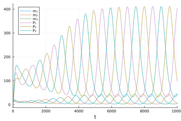
Then we can solve this reaction network

tspan = (0.0, 10000.0)
oprob = ODEProblem(repressilator, u₀, tspan, p)
sol = solve(oprob)
plot(sol)

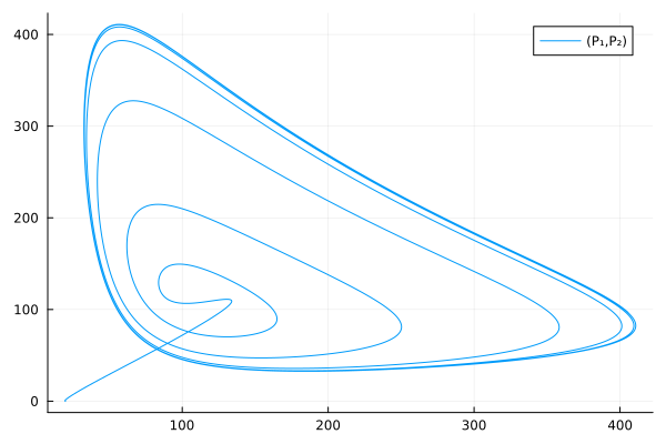
Use extracted symbols.

plot(sol, idxs=(P₁, P₂))

Convert to Stochastic Differential Equation (SDE) Models

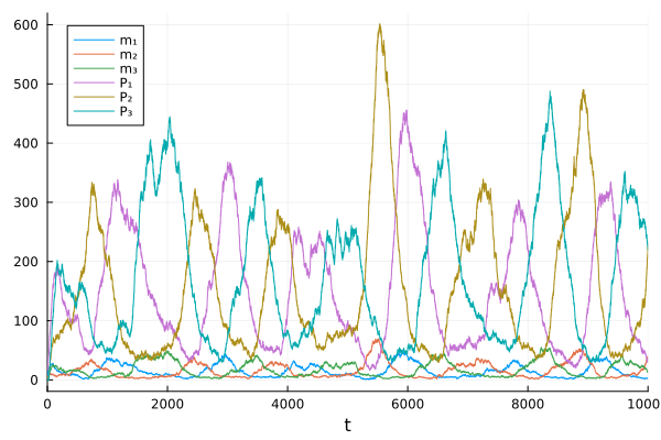
Convert the very same reaction network to Chemical Langevin Equation (CLE), adding Brownian motion terms to the state variables. Build an SDEProblem with the reaction network

tspan = (0.0, 10000.0)
sprob = SDEProblem(repressilator, u₀, tspan, p)

SDEProblem with uType Vector{Float64} and tType Float64. In-place: true
timespan: (0.0, 10000.0)
u0: 6-element Vector{Float64}:
  0.0
  0.0
  0.0
 20.0
  0.0
  0.0

tstops is used to specify enough points that the plot looks well-resolved.

sol = solve(sprob, LambaEulerHeun(), tstops=range(0.0, tspan[2]; length=1001))
plot(sol)

# Using Gillespie's stochastic simulation algorithm (SSA)

Create a Gillespie stochastic simulation model with the same reaction network. The initial conditions should be integers

u0 = [m₁ => 0, m₂ => 0, m₃ => 0, P₁ => 20, P₂ => 0, P₃ => 0]

6-element Vector{Pair{Symbolics.Num, Int64}}:
 m₁(t) => 0
 m₂(t) => 0
 m₃(t) => 0
 P₁(t) => 20
 P₂(t) => 0
 P₃(t) => 0

Create a discrete problem because our species are integer-valued:

dprob = DiscreteProblem(repressilator, u0, tspan, p)

DiscreteProblem with uType Vector{Float64} and tType Float64. In-place: true
timespan: (0.0, 10000.0)
u0: 6-element Vector{Float64}:
  0.0
  0.0
  0.0
 20.0
  0.0
  0.0

Create a JumpProblem, and specify Gillespie’s Direct Method as the solver.

jprob = JumpProblem(repressilator, dprob, Direct(), save_positions=(false, false))

JumpProblem with problem DiscreteProblem with aggregator JumpProcesses.Direct
Number of jumps with discrete aggregation: 3
Number of jumps with continuous aggregation: 0
Number of mass action jumps: 12

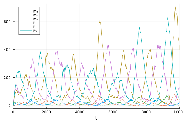
Solve and visualize the problem.

sol = solve(jprob, SSAStepper(), saveat=10.0)
plot(sol)

---

This notebook was generated using Literate.jl.