Stochastic Differential Equations (SDEs)#
SDE example in
DifferentialEquations.jlRODE example in
DifferentialEquations.jl
Stochastic Differential Equations (SDEs)#
Recommended SDE solvers: https://docs.sciml.ai/DiffEqDocs/stable/solvers/sde_solve/
Scalar SDEs with one state variable#
Solving the equation: \(du=f(u,p,t)dt + g(u,p,t)dW\)
\(f(u,p,t)\) is the ordinary differential equations (ODEs) part
\(g(u,p,t)\) is the stochastic part, paired with a Brownian motion term \(dW\).
using DifferentialEquations
using Plots
ODE function
f = (u, p, t) -> p.α * u
#1 (generic function with 1 method)
Noise term
g = (u, p, t) -> p.β * u
#3 (generic function with 1 method)
Setup the SDE problem
p = (α=1, β=1)
u0 = 1 / 2
dt = 1 // 2^(4)
tspan = (0.0, 1.0)
prob = SDEProblem(f, g, u0, (0.0, 1.0), p)
SDEProblem with uType Float64 and tType Float64. In-place: false
timespan: (0.0, 1.0)
u0: 0.5
Use the classic Euler-Maruyama algorithm to solve the problem
sol = solve(prob, EM(), dt=dt)
retcode: Success
Interpolation: 1st order linear
t: 17-element Vector{Float64}:
 0.0
 0.0625
 0.125
 0.1875
 0.25
 0.3125
 0.375
 0.4375
 0.5
 0.5625
 0.625
 0.6875
 0.75
 0.8125
 0.875
 0.9375
 1.0
u: 17-element Vector{Float64}:
 0.5
 0.575250467218189
 0.5210141807230529
 0.6087965919181457
 0.4551274785679297
 0.5353536091302965
 0.36264843958813064
 0.34757723372159377
 0.3648621176077021
 0.3045696146791805
 0.27419934436778887
 0.3563975922254598
 0.3140962460605582
 0.1702719128231658
 0.2356156758526306
 0.19742118492932542
 0.21880279007818898
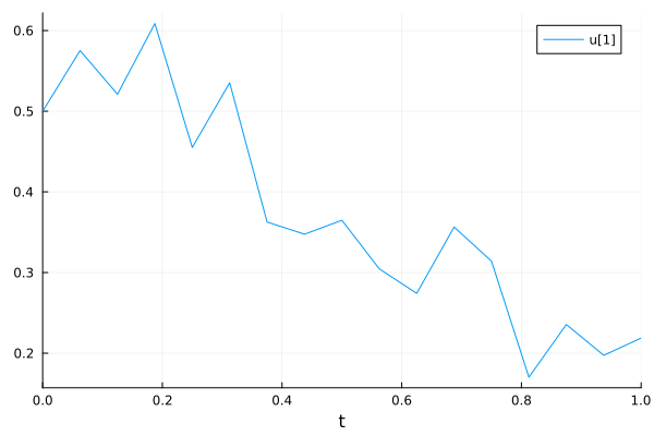
Visualize
plot(sol)
The analytical solution: If \(f(u,p,t) = \alpha u\) and \(g(u,p,t) = \beta u\), the analytical solution is \(u(t, W_t) = u_0 exp((\alpha - \frac{\beta^2}{2})t + \beta W_t)\)
f_analytic = (u0, p, t, W) -> u0 * exp((p.α - (p.β^2) / 2) * t + p.β * W)
ff = SDEFunction(f, g, analytic=f_analytic)
prob = SDEProblem(ff, g, u0, (0.0, 1.0), p)
SDEProblem with uType Float64 and tType Float64. In-place: false
timespan: (0.0, 1.0)
u0: 0.5
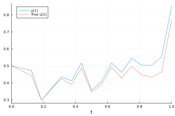
Visualize numerical and analytical solutions
sol = solve(prob, EM(), dt=dt)
plot(sol, plot_analytic=true)
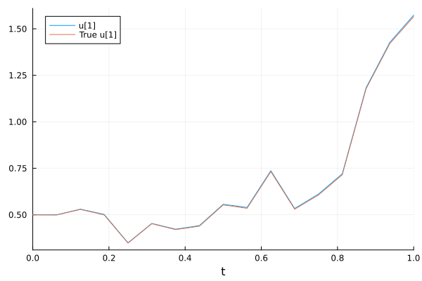
Use a higher-order solver for a more accurate result
sol = solve(prob, SRIW1(), dt=dt, adaptive=false)
plot(sol, plot_analytic=true)
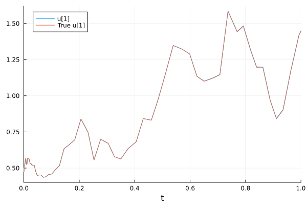
The solver is adaptive and can find dt itself
sol = solve(prob, SRIW1())
plot(sol, plot_analytic=true)
SDEs with diagonal Noise#
Each state variable are influenced by its own noise. Here we use the Lorenz system with noise as an example.
using DifferentialEquations
using Plots

function lorenz!(du, u, p, t)
    du[1] = 10.0(u[2] - u[1])
    du[2] = u[1] * (28.0 - u[3]) - u[2]
    du[3] = u[1] * u[2] - (8 / 3) * u[3]
end

function σ_lorenz!(du, u, p, t)
    du[1] = 3.0
    du[2] = 3.0
    du[3] = 3.0
end

prob_sde_lorenz = SDEProblem(lorenz!, σ_lorenz!, [1.0, 0.0, 0.0], (0.0, 20.0))
sol = solve(prob_sde_lorenz)
plot(sol, idxs=(1, 2, 3), label=false)
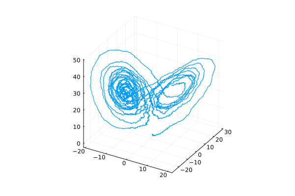
SDEs with scalar Noise#
The same noise process (W) is applied to all state variables.
using DifferentialEquations
using Plots
Exponential growth with noise
f = (du, u, p, t) -> (du .= u)
g = (du, u, p, t) -> (du .= u)
#9 (generic function with 1 method)
Problem setup
u0 = rand(4, 2)
W = WienerProcess(0.0, 0.0, 0.0)
prob = SDEProblem(f, g, u0, (0.0, 1.0), noise=W)
SDEProblem with uType Matrix{Float64} and tType Float64. In-place: true
timespan: (0.0, 1.0)
u0: 4×2 Matrix{Float64}:
 0.312443  0.841388
 0.45711   0.632634
 0.348532  0.111465
 0.990666  0.371356
Solve and visualize
sol = solve(prob, SRIW1())
plot(sol)
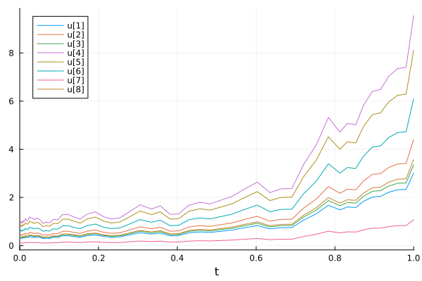
SDEs with Non-Diagonal (matrix) Noise#
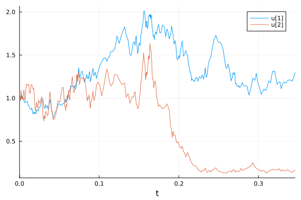
A more general type of noise allows for the terms to linearly mixed via noise function g being a matrix.
using DifferentialEquations
using Plots

f = (du, u, p, t) -> du .= 1.01u

g = (du, u, p, t) -> begin
    du[1, 1] = 0.3u[1]
    du[1, 2] = 0.6u[1]
    du[1, 3] = 0.9u[1]
    du[1, 4] = 0.12u[1]
    du[2, 1] = 1.2u[2]
    du[2, 2] = 0.2u[2]
    du[2, 3] = 0.3u[2]
    du[2, 4] = 1.8u[2]
end

u0 = ones(2)
tspan = (0.0, 1.0)
(0.0, 1.0)
The noise matrix itself is determined by the keyword argument noise_rate_prototype
prob = SDEProblem(f, g, u0, tspan, noise_rate_prototype=zeros(2, 4))
sol = solve(prob, LambaEM())
plot(sol)
┌ Warning: dt(2.220446049250313e-16) <= dtmin(2.220446049250313e-16) at t=0.3459307875829976, and step error estimate = 9.01747223517444. Aborting. There is either an error in your model specification or the true solution is unstable.
└ @ SciMLBase ~/.julia/packages/SciMLBase/BWkqx/src/integrator_interface.jl:612
Random ODEs#
https://docs.sciml.ai/DiffEqDocs/stable/tutorials/rode_example/
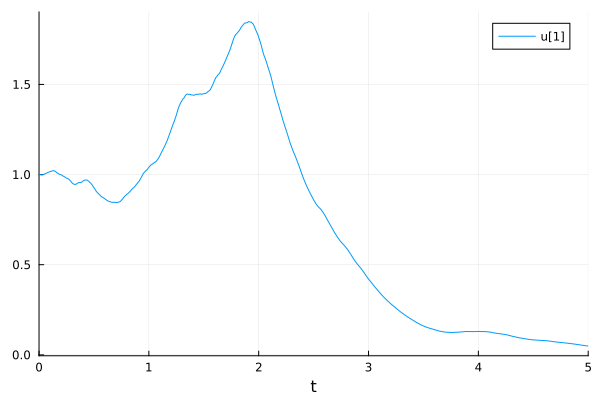
Random ODEs (RODEs) is a more general form that allows nonlinear mixings of randomness.
\(du = f(u, p, t, W) dt\) where \(W(t)\) is a Wiener process (Gaussian process).
RODEProblem(f, u0, tspan [, params]) constructs an RODE problem.
The model function signature is
f(u, p, t, W)(out-of-place form).f(du, u, p, t, W)(in-place form).
using DifferentialEquations
using Plots
Scalar RODEs
u0 = 1.00
tspan = (0.0, 5.0)
prob = RODEProblem((u, p, t, W) -> 2u * sin(W), u0, tspan)
sol = solve(prob, RandomEM(), dt=1 / 100)
plot(sol)
Systems of RODEs
using DifferentialEquations
using Plots

function f4(du, u, p, t, W)
    du[1] = 2u[1] * sin(W[1] - W[2])
    du[2] = -2u[2] * cos(W[1] + W[2])
end

u0 = [1.00; 1.00]
tspan = (0.0, 5.0)

prob = RODEProblem(f4, u0, tspan)
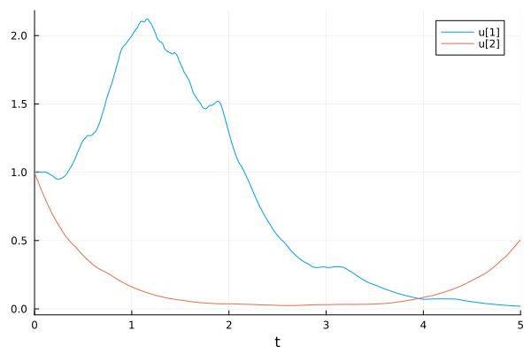
sol = solve(prob, RandomEM(), dt=1 / 100)
plot(sol)
SDEs with ModelingToolkit.jl#
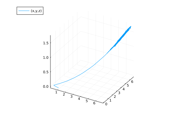
Define a stochastic Lorentz system using SDESystem(equations, noises, iv, dv, ps).
Add a diagonal noise with 10% of the magnitude, using a Brownian variable (@brownian x).
using ModelingToolkit
using DifferentialEquations
using Plots

@parameters σ ρ β
@variables t x(t) y(t) z(t)
@brownian a
D = Differential(t)

eqs = [
    D(x) ~ σ * (y - x) + 0.1a * x,
    D(y) ~ x * (ρ - z) - y + 0.1a * y,
    D(z) ~ x * y - β * z + 0.1a * z
]

@mtkbuild de = System(eqs, t)

u0map = [
    x => 1.0,
    y => 0.0,
    z => 0.0
]

parammap = [
    σ => 10.0,
    β => 26.0,
    ρ => 2.33
]

tspan = (0.0, 100.0)

prob = SDEProblem(de, u0map, tspan, parammap)
sol = solve(prob, LambaEulerHeun())
plot(sol, idxs=(x, y, z))
┌ Warning: Independent variable t should be defined with @independent_variables t.
└ @ ModelingToolkit ~/.julia/packages/ModelingToolkit/zfOUk/src/utils.jl:119
This notebook was generated using Literate.jl.
