GitLab CI/CD is a tool built into GitLab for software development for Continuous Integration (CI) and Continuous Delivery/Deployment (CD).
Test and build in parallel with matrix build in Gitlab CI/CD.
For example,
.gitlab-ci.ymltest:
image: $IMAGE
script:
- echo $MSG
- python -V
parallel:
matrix:
# First cartesian set of parameters
- IMAGE: ['python:3.6-alpine', 'python:3.7-alpine']
MSG: ['Test1', 'Test2']
# Second cartesian set of parameters
This will create 4 jobs with a combination of a custom message and a specific Python image.
See also the blog post by Michael Friedrich for more parallel matrix build with GitLab CI/CD.
GitLab CI/CD rules reference
Note
Rules cannot be used together with only/except. Otherwise, GitLab will return a key may not be used with rules error.
.gitlab-ci.ymlscheduled-update:
# only run if this is a scheduled pipeline
rules:
- if: $CI_PIPELINE_SOURCE == "schedule"
.gitlab-ci.ymlpush-job:
rules:
- if: $CI_PIPELINE_SOURCE == "push"
.gitlab-ci.ymlmerge-request:
rules:
- if: $CI_PIPELINE_SOURCE == "merge_request_event"
.gitlab-ci.yml# GitLab pages job
pages:
rules:
- if: $CI_COMMIT_BRANCH == $CI_DEFAULT_BRANCH
.gitlab-ci.ymlpages:
rules:
- if: $CI_COMMIT_TAG
Use tags to tun jobs in a specific runner e.g., your self-hosted GitLab runner in the workstation.
.gitlab-ci.ymlrun-custom:
tags:
- myWS
script:
- echo "Running in my workstation."
Create a release with GitLab CI/CD pipelines with the release-cli docker image:
.gitlab-ci.ymlrelease_job:
stage: release
image: registry.gitlab.com/gitlab-org/release-cli:latest
rules:
- if: $CI_COMMIT_TAG # Run this job when a tag is created manually
script:
- echo "Running the release job."
release:
name: "Release $CI_COMMIT_TAG"
description: "Release created using the release-cli."
We can cache conda packages by setting CONDA_PKGS_DIRS environment variable inside the project folder (CI_PROJECT_DIR) so that the GitLab runner can cache these dependencies.
.gitlab-ci.ymlimage: condaforge/miniforge3:latest
variables:
CONDA_PKGS_DIRS: "${CI_PROJECT_DIR}/.cache/conda/pkgs"
cache:
- key:
files:
- environment.yml
paths:
- .env/
- .cache/conda/pkgs
before_script:
- conda env update --prefix ./.env --file environment.yml --prune
- source activate ./.env
Because GitLab only caches files inside the project folder (CI_PROJECT_DIR)
CONDA_PKGS_DIRS is set to ${CI_PROJECT_DIR}/.cache/conda/pkgs to hold the downloaded compressed packages.- Extracted environment folder is set to
${CI_PROJECT_DIR}/.env using the --prefix option.
Conda will create the runtime environment according to environment.yml. The environment folder will be created (if not present) or cached. The option --prune means conda will remove unnecessary packages for subsequent caching.
Warning
Currently the private key cannot be masked and base64 encoding/decoding is needed.
You can use a pair of SSH keys to access a git repository
- The private key would be a CI/CD project variable
- The public key would be a deploy key
You also need additional steps to setup a SSH client in the pipeline.
before_script:
   # apt-get applies to Debian-based images. Change the package manager if needed.
  - 'which ssh-agent || ( apt-get update -qy && apt-get install openssh-client -qqy )'
  - 'which git || ( apt-get update -qy && apt-get install git -qqy )'
  - eval `ssh-agent -s`
  - echo "${SSH_PRIVATE_KEY}" | tr -d '\r' | ssh-add - > /dev/null # add ssh key
  - '[[ -f /.dockerenv ]] && echo -e "Host *\n\tStrictHostKeyChecking no\n\n" > ~/.ssh/config'
And replace the default HTTP-based git origin with the SSH one.
script:
  - git remote rm origin && git remote add origin git@gitlab.com:$CI_PROJECT_PATH.git
Compared to SSH, using a personal access token (PAT) with write repo right might be simpler. In the following example, the PAT is stored as a masked CI/CD variable GIT_PUSH_TOKEN.
script:
  - bash update.sh
  - |
    if [ -n $(git status --porcelain) ]; then
        echo "Committing updates"
        git config --global user.name "${GITLAB_USER_NAME}"
        git config --global user.email "${GITLAB_USER_EMAIL}"
        git add .
        git commit -m "Automated update: $(date '+%Y-%m-%d-%H-%M-%S')"
        git push "https://${GITLAB_USER_NAME}:${GIT_PUSH_TOKEN}@${CI_REPOSITORY_URL#*@}"
        exit;
    else
        echo "no change, nothing to commit"
    fi
For a MR pipeline, GitLab provides git push options for merge request settings.
script:
  - bash update.sh
  - |
    if [ -n $(git status --porcelain) ]; then
        echo "Committing updates"
        NEW_BR=auto-update-$(date '+%Y-%m-%d-%H-%M-%S')
        git config --global user.name "${GITLAB_USER_NAME}"
        git config --global user.email "${GITLAB_USER_EMAIL}"
        git checkout -b ${NEW_BR}
        git add .
        git commit -m "${NEW_BR}"
        git push "https://${GITLAB_USER_NAME}:${GIT_PUSH_TOKEN}@${CI_REPOSITORY_URL#*@}" \
            -o merge_request.create \
            -o merge_request.target="${CI_DEFAULT_BRANCH}" \
            -o merge_request.merge_when_pipeline_succeeds \
            -o merge_request.remove_source_branch \
            -o merge_request.title="${NEW_BR}" \
            -o merge_request.label="automated update" \
            -o merge_request.assign="${GITLAB_USER_NAME}"
        exit;
    else
        echo "no change, nothing to commit"
    fi
Assuming you have two identical repositories on GitLab and GitHub each (you can do this by importing one's repo to the other), the following steps show how to mirror GitLab repositories to GitHub with deploy SSH keys.
- In the GitLab repo, go to
Settings/Repository/Mirroring repositories and set Git repository URL as ssh://git@github.com/<namespace>/<repo>.git. e.g. ssh://git@github.com/sosiristseng/docker-python-julia.git

Warning
The GitHub button gives git@github.com:<namespace>/<repo>.git as the repo URL, one should change it to ssh://git@github.com/<namespace>/<repo>.git for GitLab to access the repository.
-
Set Mirror direction to push.

-
Set Authentication method to SSH public key. Optionally you can click Detect host keys.

-
(Optionally) check "Keep divergent refs" to prevent force pushes and/or "Mirror only protected branches" for a cleaner GitHub mirror.
- Click
Mirror repository.
- Copy the SSH public key (the middle button) and go to the GitHub mirror repo.

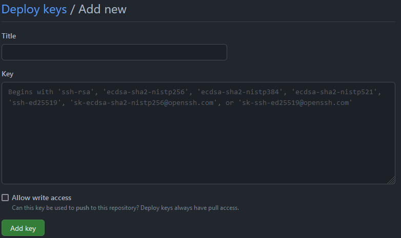
In the Github mirror repository, go to Settings/Deploy keys and add deploy key.

Paste the SSH public key copied from the GitLab source. Give it a title, allow write access, click add key to finish this step, and viola.


